Combining indirect estimates of child and adult mortality to produce a life table
Description of the method
The indirect methods described in this manual for deriving estimates of child and adult mortality produce series of estimates of child and adult mortality, which – using the time location approach pioneered by Feeney (1980, 1991) for children and Brass and Bamgboye (1981) and Brass (1985) for adults – apply to a variety of dates. In many demographic applications, however, it is useful if one can derive an abridged life table that reflects mortality over the entire age range at a specific date within the period covered by such series of indirect estimates of mortality. These applications include the production of population projections or the evaluation of changes in life expectancies at birth or mortality over time.
A general summary of the nature and range of estimates produced by the most important indirect methods is presented in Table 1.
Table 1 Indices of mortality and time references of the estimates produced by selected indirect methods for the estimation of child and adult mortality
|
Method |
Measure and typical age range |
Typical time reference |
|
Child: Indirect |
l(1) … l(20) |
1 to 15 years before the survey |
|
Adult: Maternal orphanhood |
10p25 … 40p25 |
3 to 15 years before the survey |
|
Adult: Paternal orphanhood |
15p35 … 35p35 |
5 to 15 years before the survey |
|
Adult: Siblinghood method |
10p15 … 35p15 |
3 to 15 years before the survey |
An important feature of the estimates that these methods produce for adults is that they are all conditional estimates of survivorship, that measure survival from one age (e.g., 25 in the case of the maternal orphanhood method) to another age (e.g., 35). One cannot straightforwardly convert these conditional measures of survivorship in adulthood into unconditional ones. Thus, the methods for fitting logit model life tables explained by the introductory descriptions of the models in a number of textbooks cannot be applied and more complicated fitting methods are required.
In order to combine estimates of child and adult mortality into a single life table applicable at a defined point in time, a method is needed which addresses the following list of issues:
- The adult mortality estimates need to be converted from their initial conditional form into measures of survivorship from birth
- The child and adult mortality estimates may imply different patterns or levels of mortality, different time trends in mortality, or both
- Some data points may be defective or suffer from random fluctuations that distort the overall trend, which implies that the implied trend may require smoothing or adjustment
- The estimates of child and adult mortality typically refer to different dates and may span different periods of time
- Neither the methods for estimating child mortality nor those for estimating adult mortality produce any information on the mortality of some age groups, implying that the one can only produce a complete life table by using models.
The method described here seeks to find the parameters α and β of a relational logit model life table (described in the Introduction to Model Life Tables) applicable to a specified point in time that offers the best fit to the observed data points used as inputs. Fitting a 2-parameter model is only possible if independent estimates are available of child and adult mortality for the date in question. If such data are available, fitting a 2-parameter model is recommended because no justification usually exists a priori for making the assumption that the age pattern of mortality in the population in question corresponds to that in any particular 1-parameter family of model life tables.
Starting with the observed quantities from the child and adult estimation, the method first derives and plots the implied values of α (the level parameter of a relational model life table) against the time location of each estimate, separately for child and adult mortality making the assumption that β (the shape parameter) is equal to 1. This ‘alpha plot’ is used to identify which data points describe a coherent and consistent trend in the value of α over time. The selected points are then used to iteratively calculate final estimates of α and β at the date for which the life table is required. A fitted model life table can then be calculated from the standard using these values of α and β. The method allows both the α and β parameters of the fitted models to change over time but constrains them to do so linearly (Timæus 1990).
The method can be used to derive abridged life tables from sex-specific estimates of child mortality produced by the indirect method for the analysis of data on women’s children ever-born and still alive, and sex-specific estimates of adult mortality produced by application of either the One Census Orphanhood or Indirect Siblinghood methods. Estimates of child and adult mortality made by direct methods, or from the application of two-census methods, normally apply to a specific year or period of time. Model life tables can be fitted to pairs of estimates of adult and child mortality that refer to the same calendar time using the methods described in the section on fitting life tables to a pair of estimates of childhood and adult mortality.
Data requirements and assumptions
Tabulations of data required
- A series of sex-specific indirect estimates of child mortality, with their time locations, derived from data on women’s children ever born and surviving
- A series of sex-specific estimates of adult mortality, with their time locations, derived using either the indirect method for analyzing data on sibling survival or the one census orphanhood method.
In principle, the approach used to fit such data could be extended to estimate life tables for populations for which multiple overlapping sets of indirect estimates exist describing child and adult mortality. However, the accompanying worksheet has only been designed to handle two series of estimates: one for children and one for adults.
Assumptions
The method described here bases the fitted model life table on a standard life table. This standard is assumed to have an age pattern of mortality that resembles that of the population being studied. In particular, the relative severity of child and adult mortality in the standard should be similar to that indicated by the indirect estimates to which the model is being fitted. Guidelines for choosing an appropriate standard life table are provided in the Introduction to Model Life Tables, which also describes the basic mechanics of the relational logit system of model life tables. The standard need not be taken from the family of model life tables that underlies the coefficients that were used to produce the indirect estimates of child mortality: the family of models that best represents the age pattern of mortality within childhood may not be the family that best represents the relative levels of child and adult mortality in the same population.
Caveats and warnings
The plausibility of the fitted model life table produced by this method of fitting depends on whether the chosen standard life table is appropriate for the population under study. In populations affected by HIV/AIDS, for example, both the balance between child and adult mortality and the detailed age pattern of mortality differ greatly from those that characterize the systems of model life tables in widespread use. Consequently, this method is not recommended for routine application in these circumstances or to other populations for which no standard life table can be identified that describes the balance between child and adult mortality.
Application of method
The method is implemented using the following steps.
Step 1: Identify the date to which the desired life table should apply
To avoid the risks associated with out-of-sample extrapolation in the determination of α and β, the life table should be fitted to a date within the period covered by the estimates of adult and child estimates that are being analyzed. In the presentation of the method that follows, this target date is denoted by D.
The exact date for which the life table is required may be determined by the use to which it is going to be put. Ideally a date should be chosen, however, for which both the estimates of adult and child mortality seem reliable. For example, if either the more distant estimates for children appear to biased downward by underreporting of dead children or the more recent estimates for adults appear to be biased downward by the adoption effect, one should avoid producing a life table for the dates covered by the defective estimates. Unfortunately, such considerations sometimes lead the analyst to the conclusion that the data at hand fail to provide a sound basis for the construction of a life table!
If a life table is needed for a more recent, or possibly a more distant, date than the period of time covered by the estimates, a limited amount of extrapolation beyond this range of dates might be considered. The extent of this should be restricted to three years before the earliest time location of any adult or child mortality estimates, on the one hand, and to three years after the earlier of the most recent estimate of child mortality and the most recent estimate of adult mortality, on the other.
Step 2: Select a standard to be used to derive the fitted life table
The associated spreadsheet allows the analyst to choose between nine sex-specific standards: the five UN model life tables (General; South Asian; Far Asian; Latin American; Chilean) and the four Princeton regional model life tables (North; South; East; West). All the standard life tables have a life expectancy at birth of 60 years. The derivation of these logits is described in the Introduction to Model Life Tables, and a spreadsheet containing their values can be downloaded from the Tools for Demographic Estimation website.
The primary objective in selecting a standard should be to identify one in which the relationship between child and adult mortality is approximately the same as that indicated by the estimates of child and adult mortality. As a practical rule of thumb, if the value of β of the final fitted model lies outside the range 0.75-1.25, one should at least consider adopting another standard. In more extreme circumstances, model life tables in which β falls outside the range 0.6-1.4 are unlikely to represent empirical mortality schedules adequately. A secondary objective in choosing a standard should be to identify one that shares other known characteristics of the population in question such as the relationship between infant mortality and mortality at ages 1 to 4. The characteristics of the different Princeton and UN families of model life tables are described briefly in the Introduction to Model Life Tables.
Step 3: Plot values of α (assuming β = 1) derived from the mortality estimates against time
When β (the shape parameter in a relational model life table system) equals 1, the relational model life table system can be expressed as
where Y(x) is the logit transform
For child mortality, calculating a series of values of α from the estimates is straightforward. The logits of the chosen standard life table for ages 1, 2, 3, 5, 10, 15 and 20 are subtracted from the logits of the derived estimates of child mortality (q(1), q(2), q(3), q(5), q(10), q(15) and q(20)):
For adults, the calculation of α is more complicated as the survival probabilities produced by the estimation methods are conditional on survival to a given base age. The formula for α is
where x is the base age of the conditional probability of survival (25 for the maternal orphanhood method) and n is the duration over which survivorship is measured, which is contingent on the age group of the respondent. (The derivation of this expression can be found at the end of this page).
The estimates of α (separately for children and adults) are then plotted against their respective time locations on the same set of axes.
Step 4: Eliminate those points in the alpha plot that appear out of line with the general trend
In order to estimate α and β for a specific point in time, the method imposes a linear trend on both parameters. As the first step to achieving this goal, we would like the plots of each of the series of α’s (that is, for children and adults separately) against their time locations derived in Step 3 to lie on straight lines.
The α’s for individual data points in a series of child or adult mortality estimates derived using the two formulae above may deviate from a straight line for several reasons. First, the underlying pattern of change in mortality may have been strongly non-linear. This is somewhat unlikely given that the series of estimates cover fairly short periods of time and that indirect estimation methods tend to smooth out short term fluctuations in mortality. Even if the diagnostic plot derived above suggests that it is the case, it may still be possible to obtain an adequate fitted model life table by calculating it for a date at which the linear trends in the parameters imposed by the method intersect with the curve indicated by the plotted points. Second, the series may be rather erratic due to sampling errors and reporting errors such as age misstatement. If this is the only limitation of the estimates, one would normally include them all in the analysis and rely on the line fitting procedure to average across these fluctuations.
Third, indirect estimates are vulnerable to biases resulting from respondents failing to answer the key questions accurately or to breaches in the assumptions of the methods concerned. Likely errors in the estimates are discussed in the pages on the various methods and the reader is referred to those pages for advice on diagnostic signs that may suggest indicate certain points are biased and should be dropped from the fitting procedure. It is particularly common, however, for the point relating to respondents aged 15-19 in the child mortality method to be biased upward and for the points relating to children aged 5-14 reporting on the survival of their parents in the one census orphanhood method to be biased downward. It will often be necessary to exclude these data points from the model fitting process.
A fourth possible explanation for the failure of the calculated α’s to lie on a straight line is that the standard selected for calculating the original estimates may not have been appropriate. If this is the case, it may be necessary to recalculate these estimates using a different standard. Alternately, it may be necessary to try using an alternative standard (as described in Step 2) to derive the fitted life table.
Once the child and adult α’s for inclusion in the fitting process have been selected, the rest of the fitting process proceeds mechanically.
Step 5: Determine the trend in β by iteration
The process of solving for β iteratively is not readily done manually, and the associated workbook has been designed to perform the calculations. In order to enable the iteration routine, ensure that Microsoft Excel has been configured appropriately. This is done by selecting "File → Options → Formulas and then checking the “Enable iterative calculation” checkbox. Setting a maximum of 1000 iterations and a maximum change of 0.00001 is more than sufficient for a solution to be reached.
The process whereby β and α are adjusted iteratively to secure a good fit is described in the section on the Mathematical Exposition of the method. The key constraints placed on the fitting process are as follows:
- No matter what the original values of x and n in the estimates of q(x) and npb for children and adults respectively at the date in question, β is calculated consistently from survivorship from age 15 to 60 relative to the standard.
- Both α and β are allowed to change over time but it is assumed that they do so linearly.
In combination, these assumptions reduce the distorting impact that errors in the estimates and minor differences in the age pattern of mortality between the population and the standard can have on the fitted model life table (Timæus 1990). In contrast, if one uses the method described elsewhere to fit a 2-parameter logit model life table to a pair of recent indirect estimates of child and adult mortality that refer to about the same date but only measure mortality over a limited range of ages (Brass 1975, 1985), for example q(2) and 10p25, one frequently obtains extreme values of β that produce implausible fitted models.
Step 6: Examine the resulting fitted values of α
The penultimate step is to examine the alpha plot that results from the iterative fitting procedure, which is presented as the second plot of the alpha plots sheet of the associated workbook. It is this plot, which presents estimates of α that have been adjusted for the level and trend in β, that provides a check on the assumption that α has followed a linear trend. Moreover, if the standard to which the data have been fitted is appropriate, the series of estimates of childhood and adult mortality should lie close to each other in this plot.
Step 7: Production of a fitted life table
Once the best fitting linear time trends in α and β have been identified by the iterative fitting process, fitted values of α and β for the date for which a fitted life table is required, D, are calculated as follows:
The abridged fitted life table is derived from these values of α* and β* and the standard life table by means of the formula
Worked example
The worked example presented here uses data on the female population from the Dominican Republic. The indirect estimates for girls were made from the data on children ever-born and surviving obtained by a DHS conducted in 2002. The indirect estimates for adult women were made from the reports on the survival of mothers from the census conducted in the same year. The input data are presented in Table 2.
Table 2 Input data for combining child and adult mortality estimates, Dominican Republic
|
Child mortality (2002 DHS) |
|
Adult mortality (2002 Census) |
||||
|
x |
q(x) |
Date |
|
n |
np25 |
Date |
|
1 |
0.0338 |
2001.71 |
|
10 |
0.9858 |
1999.23 |
|
2 |
0.0429 |
2000.24 |
|
15 |
0.9801 |
1997.07 |
|
3 |
0.0355 |
1998.48 |
|
20 |
0.9680 |
1995.13 |
|
5 |
0.0467 |
1996.43 |
|
25 |
0.9479 |
1993.43 |
|
10 |
0.0619 |
1994.16 |
|
30 |
0.9214 |
1992.02 |
|
15 |
0.0710 |
1991.52 |
|
35 |
0.8872 |
1991.00 |
|
20 |
0.0799 |
1987.99 |
|
40 |
0.8373 |
1990.51 |
Step 1: Identify the date to which the desired life table should apply
In the case of the data from the Dominican Republic, the associated spreadsheet permits a life table to be derived for dates lying between the earlier of 1987.99-3 and 1990.51-3 and the earlier of 2001.71+3 and 1999.23+3, which is to say dates between 1984.99 and 2002.23.
In this example, we derive a life table for the Dominican Republic for mid-1997, i.e. 1997.5.
Step 2: Select a standard to be used to derive the fitted life table
Given the geographical source of the data, it is reasonable to assume (at least initially) that the mortality of women in the Dominican Republic follows the age pattern described by the UN Latin American female standard. The logits of the chosen standard life table are presented in Table 3.
Table 3 Logits of the UN Latin American female life table with a life expectancy of 60 years
|
Age (x) |
Ys(x) = logit(l(x)) |
|
0 |
|
|
1 |
-1.2375 |
|
2 |
-1.1006 |
|
3 |
-1.0398 |
|
4 |
-1.0046 |
|
5 |
-0.9815 |
|
10 |
-0.9304 |
|
15 |
-0.9054 |
|
20 |
-0.8735 |
|
25 |
-0.8313 |
|
30 |
-0.7828 |
|
35 |
-0.7285 |
|
40 |
-0.6670 |
|
45 |
-0.6005 |
|
50 |
-0.5248 |
|
55 |
-0.4356 |
|
60 |
-0.3230 |
|
65 |
-0.1795 |
Note that, if you change the family of life tables from “UN” to “Princeton” or vice versa in the associated workbook, you must force the workbook to recalculate the output by changing the “Recalculate” cell (B3 on the Method sheet) from “True” to “False” and back to “True”. Failure to do this will produce an error.
Step 3: Plot values of α (assuming β=1) derived from the mortality estimates against their time locations
Using the data from the Dominican Republic in Table 2 and a UN Latin American life table for a standard, the value of α for child mortality when x = 3 is derived as follows:
This value of α has a time location of 1998.48, as indicated in Table 1. The values of α for the other estimates of child mortality, together with their time locations are derived similarly.
Using the data on adult mortality in Table 2 and the same standard, the estimate of the adult α when n is 25 is given by
This value of α has a time location of 1993.43. The values of α for the other estimates of adult mortality, together with their time locations are derived similarly.
A summary of these estimates of α and their time locations are presented in Table 4.
Table 4 Estimates of α and the time location of the estimates, Dominican Republic, 2002
|
Children |
|
Adults |
||||
|
Original index |
α |
Time location |
|
Original index |
α |
Time location |
|
q(1) |
-0.4389 |
2001.71 |
|
10p25 |
-0.5176 |
1999.23 |
|
q(2) |
-0.4519 |
2000.24 |
|
15p25 |
-0.6183 |
1997.07 |
|
q(3) |
-0.6112 |
1998.48 |
|
20p25 |
-0.5779 |
1995.13 |
|
q(5) |
-0.5266 |
1996.43 |
|
25p25 |
-0.5021 |
1993.43 |
|
q(10) |
-0.4288 |
1994.16 |
|
30p25 |
-0.4567 |
1992.02 |
|
q(15) |
-0.3803 |
1991.52 |
|
35p25 |
-0.4463 |
1991.00 |
|
q(20) |
-0.3483 |
1987.99 |
|
40p25 |
-0.4436 |
1990.51 |
When all the estimates of α based on data on both children and adults are plotted against their time locations, the alpha plot shown in Figure 1 results.
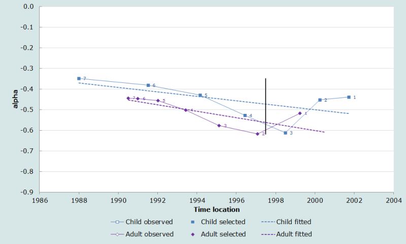
Step 4: Eliminate those points in the alpha plot that are out of line with the general trend
The section on indirect estimation of child mortality explains that the most recent indirect estimate of child mortality, which is based on the reports of women aged 15-19 tends to be biased upward as teenage mothers are a select group with high mortality because, among other reasons, they tend to come from socially disadvantaged backgrounds. This data point is nearly always ignored when inferences are made about the trend in child mortality from indirect estimates and this was done in this application.
The most recent estimate of adult mortality based on children aged 5-9 reporting on the survival of their mothers in the one census orphanhood method also underestimates mortality in many applications. In the Dominican Republic, however it indicates much higher mortality than one would expect given the trend indicated by the other estimates for adult women. This might be the result of severe underreporting of the ages of children or might indicate that the models involved in the estimation process are inappropriate for this population. Either way it was decided to ignore this anomalous estimate. Therefore, the most recent estimate in each series was omitted from the fitting of a trend line to the α’s by clearing its respective cell in the alpha plots sheet of the associated workbook.
The remaining estimates from the orphanhood method are internally consistent and suggest that adult women’s mortality fell rapidly in the Dominican Republic during the 1990s. The child mortality estimates also suggest that mortality was falling, but the more recent estimates are somewhat inconsistent with each other. The 3rd and 4th points, which are based on the reports of mothers aged 25-34 years, indicate that the rate of decline in child mortality accelerated in the second half of the 1990s. However, the 2nd estimate, which is based on the reports of women aged 20-24, suggests that it decelerated. In the absence of evidence as to the nature of the errors in the data that have led to these inconsistencies, it was decided to leave all three data points in the analysis.
The final selection of points produces the alpha plot in Figure 2. This plot emphasizes the consistency of the 2nd to 7th points for adults and shows that a regression line fitted to the 2nd to 7th points for children not only passes through the middle of the more recent estimates, but fits the three more distant points well.
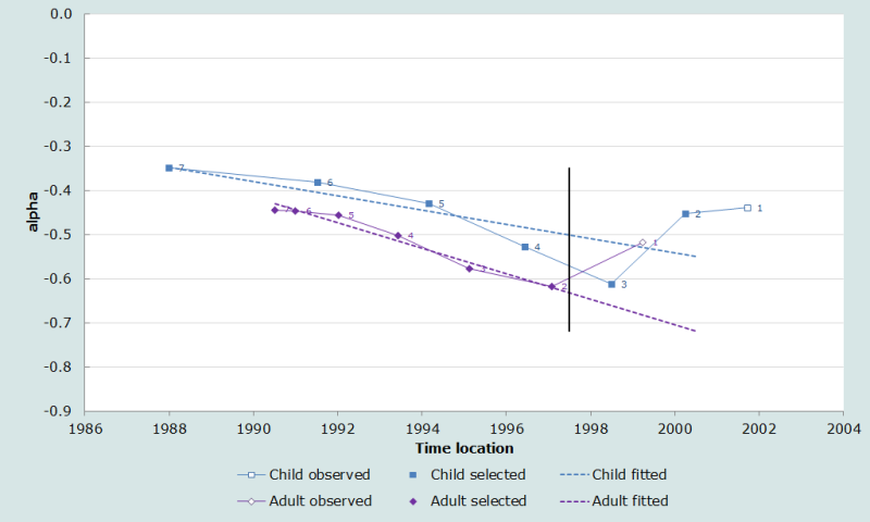
Note that, in Figure 2, the values of α derived from the estimates of the mortality of adults lie below those derived from the estimates of child mortality and diverge from them over time. This means that, relative to the UN Latin American standard, adult mortality in the Dominican Republic in the 1990s was low and was falling more rapidly than child mortality. Thus, the β parameter of fitted model life tables for this population will lie below 1 and will decrease over time.
Step 5: Determine the trend in β by iteration
The spreadsheet iteratively solves for fitted values of both α and β for the desired time point (1997.5). The estimates of α* and β* are -0.658 and 0.849 respectively. These estimates implies that the level of mortality in the Dominican Republic is somewhat lighter than in the UN Latin American standard (α < 0), and that mortality is somewhat heavier at younger ages and lighter at older ages (β < 1) than in this standard. The estimate of β* is close enough to 1 not to raise any concerns about the choice of standard made in Step 2.
Step 6: Examine the resulting fitted values of α
The penultimate step is to examine the alpha plot that results from the iterative fitting procedure, which is presented as the second plot of the “alpha plots” sheet of the associated workbook.
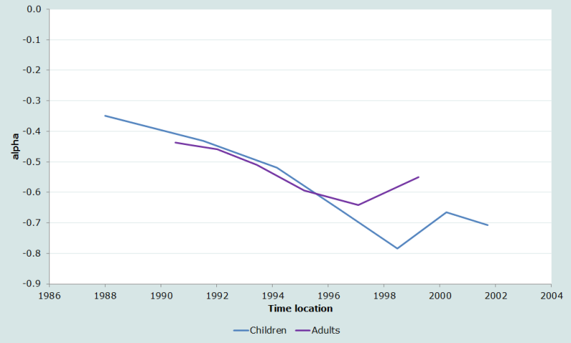
Figure 3 shows that there is now a close correspondence between the α’s for children and adults for most of the 1990s. Mortality was falling across the age range, though β dropped from about 0.95 to 0.85 between the early 1990s and mid-1997. This is what one would expect given that we have already observed that adult mortality in the Dominican Republic was falling rapidly at this time in comparison with the pattern in the family of logit model life tables based on the UN Latin American standard.
The lines for adults and children remain fairly close to each other in 1997, reflecting the fact that the value of β at that time (i.e., 0.85) remained fairly close to its central value of 1. The two estimates of α for 1997 would only differ greatly if β at this time was very different from 1. If they did differ markedly, it would be advisable to seek out a standard life table that was more appropriate for the population being studied.
If the two series of estimates followed very different trends and failed to cross over each other, or did so and then diverged rapidly, or if one or both series were highly non-linear, this would again suggest that the standard being used was inappropriate or, more probably, that one or both series was severely biased by errors in the data, making it impossible to reconcile them with each other.
Step 7: Production of a fitted life table
The abridged fitted life table is derived from the fitted values of α* = -0.658 and β* = 0.849 for the selected date, and the standard life table (presented in Table 3) by means of the formula
The final fitted life table is presented in Table 5. Life expectancy at birth is 76.6 years compared with the United Nations’ estimate for the same quinquennium of 73.1 years (UN Population Division 2013).
Table 5 Fitted life table for females, Dominican Republic, mid-1997
|
Age (x) |
l(x) |
|
0 |
1.0000 |
|
1 |
0.9683 |
|
2 |
0.9603 |
|
3 |
0.9561 |
|
4 |
0.9536 |
|
5 |
0.9518 |
|
10 |
0.9476 |
|
15 |
0.9455 |
|
20 |
0.9426 |
|
25 |
0.9386 |
|
30 |
0.9337 |
|
35 |
0.9278 |
|
40 |
0.9204 |
|
45 |
0.9118 |
|
50 |
0.9008 |
|
55 |
0.8865 |
|
60 |
0.8657 |
|
65 |
0.8348 |
|
70 |
0.7863 |
|
75 |
0.7120 |
|
80 |
0.6029 |
|
85 |
0.4452 |
|
90 |
0.2587 |
|
95 |
0.1024 |
|
100 |
0.0242 |
Detailed description of the method
The associated spreadsheet implements the method by following the steps outlined above. This section provides a detailed description of how the iterative procedure used to derive the final values of α and β is implemented.
The premise underlying the fitting procedure is that the derived life table should fit the observed data well at ages 15 and 60. The former constraint ensures that child and adolescent mortality is well matched; the combination of the two ensures that adult mortality over an extended age range (15 to 60) is close to that implied by the adult mortality estimates used to fit the life table.
Fitting procedure
After selecting the data points that will be used (as described in Step 4), the method seeks to find the best fitting linear regression model of the time trend in the estimates of α for children, conditional on the estimated trend in β, and the best fitting linear regression model of the time trend in the estimates of β for adults, conditional on the estimated trend in α for children.
Starting with the assumption that β = 1, one can calculate an αchild corresponding to each estimate of child mortality using the equation provided in Step 3 of the worked example. Since each estimate of αchild is associated with its time location (T), one can regress the estimates included in the fitting procedure on time to obtain the slope S(α) and intercept Z(α) of the linear regression model.
The fitted regression model can then be used to predict a fitted α (α*) for the times to which the adult mortality estimates refer
Using these fitted values of αchild, one can estimate Y(15) at these dates
where, in this first iteration, β* = 1.
Still assuming that β = 1, one can also estimate αadult from the conditional estimates of adult survivorship that have been included in the fitting procedure using the equation given in Step 3 of the worked example and use these values of αadult to calculate corresponding estimates of 45q15. Multiplying the value of l(15) estimated from the data on children by an estimate of 45p15 for the same date estimated from the data on adults gives an unconditional estimate of l(60) and therefore of Y(60):
The estimate of l(15) is calculated from Y(15) as
while that of 45p15 is derived from the α’s and β’s fitted to the adult estimates:
where Y s(x) represents the logit of l(x) in the standard life table (i.e., with β = 1 and α = 0) and, in this first iteration, β* = 1.
Having estimated a series of values for Y(60) for the dates to which the adult mortality estimates refer, it is now possible to calculate revised estimates of β for these dates
As these revised β’s each refer to a specific date, they can then be regressed on time (T) to calculate the slope S(β) and intercept Z(β) of a linear regression line that can then be used to predict a fitted β ( β* ) for each data point, whether it is for children or adults, from that point’s time location (T)
At this point, the first iterative cycle has been completed. One can now calculate revised estimates of αchild, that allow for the fact that β has been allowed to differ from 1, with the formula
The revised estimates of αchild are then regressed on time and used, in combination with the fitted estimates of β for the dates to which the adult mortality estimates refer, to calculate revised estimates of Y(15), 45q15 and Y(60) and then to recalculate a second round of revised estimates of β itself. Thus, we now have in place a mechanism that will iteratively calculate the best fitting regressions of α and β on time, each adjusted for the other.
Derivation of the formula for calculating α for adults
References
Brass W. 1975. Methods for Estimating Fertility and Mortality from Limited and Defective Data. Chapel Hill: International Program of Laboratories for Population Statistics.
Brass W. 1985. Advances in Methods for Estimating Fertility and Mortality from Limited and Defective Data. London: London School of Hygiene & Tropical Medicine.
Brass W and EA Bamgboye. 1981. The Time Location of Reports of Survivorship: Estimates for Maternal and Paternal Orphanhood and the Ever-widowed. London: London School of Hygiene & Tropical Medicine.
Feeney G. 1980. "Estimating infant mortality trends from child survivorship data", Population Studies 34(1):109-128. doi: https://dx.doi.org/10.1080/00324728.1980.10412839
Feeney G. 1991. "Child survivorship estimation: Methods and data analysis", Asian and Pacific Population Forum 5(2-3):51-55, 76-87. https://hdl.handle.net/10125/3600.
Timæus IM. 1990. "Advances in the Measurement of Adult Mortality from Data on Orphanhood." Unpublished PhD thesis, London: University of London. https://doi.org/10.17037/PUBS.04653370
UN Population Division. 2013. World Population Prospects: The 2012 Revision. New York: United Nations, Department of Economic and Social Affairs. https://www.un.org/development/desa/pd/sites/www.un.org.development.desa.pd/files/files/documents/2020/Jan/un_2012_world_population_prospects-2012_revision_volume-i_comprehensive-tables.pdf
- Printer-friendly version
- Log in to post comments