The Preston-Coale method

Description of method

The Preston and Coale method (Preston, Coale, Trussell et al. 1980) is the second of what later became known as the Death Distribution Methods for estimating the completeness of the reporting of deaths relative to an estimate of the population at one point in time. It makes use of the observation that the number of people of a given age alive at a point in time must be equal to the number of people from that cohort who die from that point in time onward. If the population is stable (i.e. a population with an unchanging age distribution – at least for adult ages – growing at a constant rate, r, each year) and closed to migration, and the reported data are accurate, the number of deaths aged x, t years in the future, will equal the number of deaths aged x currently, multiplied by $$e^{rt}$$. It is thus possible to estimate the current population aged y using only current deaths by age above age y and the stable growth rate r. If the number of current deaths is under-reported, but can be assumed to be under-reported to the same extent, c, at every age, then the estimate of the future number of cohort deaths will be underestimated to the same extent. Thus, it is possible to estimate the completeness of reporting of deaths by dividing the sum of the estimates of future cohort deaths derived from the number of deaths at any date by the population at the same date. Mortality rates can then be estimated by dividing the numbers of deaths reported in each adult age group by c and then dividing these numbers by an estimate of the population exposed to risk.

The method is a particular case of the more general Synthetic Extinct Generations method, which requires estimates of the population at two points in time but does not require that the population is stable. Readers are referred to that section for further detail on the method. It is included in this manual as a method that might be considered when one has an estimate of population numbers at only one point in time.

Data requirements and assumptions

Tabulations of data required

• Number of deaths of women (men), by five-year age group, and for open age interval A+ (with A as high as possible), over a specific period.
• Number of women (men), by five-year age group, and for open age interval A+, at or close to the period over which the deaths were measured.

Important assumptions

• The population is stable, although this assumption can be relaxed to some extent (see below).
• The completeness of reporting of deaths is the same for all ages above a minimum age (usually age 15).
• The population is closed to migration, although this assumption can be relaxed if net migration is small relative the mortality rates, or if one has reasonably accurate estimates of the number of migrants by age to allow for in the balance equation (which is very seldom the case).

Preparatory work and preliminary investigations

Before applying this method, you should investigate the quality of the data at least in the following dimensions:

• age structure of the population;
• sex structure of the population;
• age structure of the deaths; and
• sex structure of the deaths.

Caveats and warnings

In applying this method, analysts must take particular care with the following.

• The interpretation and estimation processes need to take into account the source of death data (vital registration, reported by households in censuses, or deaths in hospitals) as explained below.
• If applying the method to sub-national geographic areas, the issue of migration typically becomes a greater concern.
• Deciding the age range which is to be used to determine the growth rate (i.e. such that the age-specific estimates of completeness minimize the absolute difference from the mean estimate of completeness). Issues here are whether the best estimate of the growth rate to use is the intercept determined as a result of applying the Brass Growth Balance method to the same data (which would be the case if completeness was thought to decrease among the elderly, perhaps associated with retirement), and whether to exclude ages below 30 or 35 because of the impact of migration which has not been allowed for specifically.
• Deciding on the age range to use for determining the estimate of completeness. Typically, this range might exclude young adults if there is significant unaccounted-for migration, and old people if the results suggest that fewer of their deaths are reported than deaths of younger adults.
• Ensuring that the Solver routine in Excel has run satisfactorily (i.e. has produced a sensible result). Occasionally Solver offers a solution which is manifestly too low. In such situations it is best to adjust delta manually in the right direction and apply Solver to this new starting value.
• Ensuring that the estimate of life expectancy at the age of the open interval is reasonable. Often the data on older people are scanty and particularly prone to errors. Thus, estimates of life expectancy based on these data can be implausible (usually too high).
• If completeness of reporting of deaths appears to be less than 60 per cent, then caution is advised in applying this method as the uncertainty about the estimate is large.

Application of method

The method is applied in the following steps.

Step 1: Set the initial growth rate

The growth rate can be estimated initially either from estimates of the total population above a certain age (chosen to best match the assumption that population is stable) at two time points or as estimated from the application of the Brass Growth Balance method. In the first instance, if one has estimates of the total population at time points t₁ and t_2, one would estimate the growth rate as follows:

$$r=\frac{\ln \left({\text{}}_{\infty }{N}_x(t_2)/{\text{}}_{\infty }{N}_x(t_1)\right)}{t_2-t_1}$$

where $${}_{\infty }{N}_x(t)$$ is the population aged x and older at time t.

Step 2: Estimate the life expectancy at age A and five-year age intervals down to 65

This can be done in one of several ways.

1. Use estimates from an independent source if reliable estimates are available. Possible sources would be estimates produced by previous research or from population projections such as the World Population Prospects (UN Population Division 2011).
2. Use the estimates derived from the data after applying the Brass Growth Balance method. The workbook implementing that method produces such estimates as part of the output.
3. Use the ratio of the reported deaths in the age group 10 to 39 last birthday to those in the age group 40 to 59 last birthday (₃₀D₁₀/₂₀D₄₀) to determine (by comparison) a level of the West model life table, from which estimates of life expectancy can be read. These estimates are included as part of the workbook implementing this method. Unfortunately, since the West model life table does not reflect mortality resulting from HIV/AIDS, this approach is unsuitable for countries that have significant numbers of AIDS deaths.
4. Solve for the life expectancy iteratively by starting with a reasonable guess such as one estimated from the West table (although in some cases this may not work in countries with significant numbers of AIDS deaths) or from an independent source. Then estimate completeness (as described below), copy the life expectancies from the Life expectancies spreadsheet of the associated workbook, paste the values into the Method spreadsheet of the associated workbook and re-estimate completeness. Repeat if necessary until the change to life expectancies is no longer significant. Unfortunately, if there are reasons for suspecting that, even after correcting the rates for incompleteness, mortality is underestimated at the older ages (for example, if there is significant age exaggeration, or relatively higher incompleteness at the older ages) this approach will overestimate the life expectancies and hence overestimate the overall level of completeness of reporting.

Step 3: Estimate the number of people who turned x, and the number aged x to x+4 last birthday, from the reported deaths

The number of people who turned x during the period over which the deaths were reported is estimated from the reported deaths as follows:

$${\widehat{N}}_x={\widehat{N}}_{x+5}\exp \left(5r\right)+{\text{}}_5{D}_x\exp \left(2.5r\right)$$

and

$${\widehat{N}}_A={\text{}}_{\infty }{D}_A\left(\exp \left(r\times e_A\right)-{\left(r\times e_A\right)}^2/6\right)$$

where A is the age at the start of the open interval, r is the annual population growth rate, and e_A is the life expectancy at age A.

The number of people who were aged between x and x+4 last birthday during the period over which the deaths were reported is estimated from the numbers who turned x in five-year steps as follows:

$${}_5{\widehat{N}}_x=2.5\left({\widehat{N}}_x+{\widehat{N}}_{x+5}\right).$$

Step 4: Estimate the number of people who were aged x to x+4 last birthday during the period over which the deaths are reported, from the census population

The number of people who were aged x to x+4 last birthday during the period over which the deaths are reported is estimated from the census population by simply multiplying the numbers in the population in that age group by the length of the period over which the deaths are reported (measured in years).

Step 5: Calculate the ratios of the estimates of the population aged x to x+4 last birthday and the ratios of the population aged x to A-1 last birthday derived from deaths to those derived from the census population

Two sets of ratios of the estimates derived from the deaths to those derived from the census population are calculated. The first is the ratios in quinquennial age groups, which are calculated directly. The second is the ratios of the numbers from age x to that age of the open interval, A, with the numbers of people who turned x to A-1 during the period being calculated as the aggregate of the numbers in five-year age groups between ages x and A-5. In other words,

$${}_{A-x}{\widehat{N}}_x={\displaystyle \sum _{a=x,5}^{A-5}{}_5{\widehat{N}}_x}$$

Step 6: Estimate the completeness of reporting of deaths

In order to determine the level of completeness of reporting one first needs to decide if the initial choice of growth rate is correct. The interpretation of the plots of the ratios is discussed in more detail below. However, essentially the correct growth rate is identified as that which produces the most level set of ratios by age. The Method spreadsheet is set up so that Solver (Data, Solver, Solve) will find the growth rate that minimizes the absolute deviation from the mean of the ratios over the age range specified by the user.

If the initial estimate of the growth rate produces a level series of ratios across adult ages but with significant curvature downward at the older ages this could indicate a fall off in completeness at the older ages (as might be the case if, for example, people retired from urban areas to rural areas, where completeness of registration was lower). In such a situation it is important not to set the growth rate to produce a level set of ratios, but rather to use the initially chosen growth rate.

If one is also solving for the both growth rate and life expectancies iteratively, these values will need to be pasted from the Life expectancies spreadsheet into the Method spreadsheet and a new growth rate set. This process may need to be repeated two or three times, until there is no change in the life expectancies.

Finally, one decides on the age range of ratios to be used to determine the completeness. If there is a significant curvature upward at the older ages this probably indicates age exaggeration, particularly for deaths, and one needs to try and identify an age for the open interval below which the age exaggeration is not significant. If completeness drops off at ages below 35, this could indicate unaccounted for out-migration. If this is suspected then one should exclude these ages from determining the growth rate or completeness.

Completeness is estimated from the age group-specific ratios. In order to produce a robust estimate, it is calculated as the sum of 50 per cent of the median plus 25 per cent of each of the 75^th and 25^th percentile of these ratios.

However, since this is an estimate of the completeness on the assumption that the census population was at the mid-point of the period over which the deaths have been recorded, it is desirable to correct for any difference between the time of the census and the mid-point of the period over which the deaths were recorded. In order to do this we multiply this estimate of completeness by the ratio of the census population to the estimate of the population at time t_m, on the assumption that the population, which is assumed to be stable, is growing at an annual growth rate estimated by a, i.e. $$\text{}\exp \left(a\left(t_c-t_m\right)\right)$$ where t_c is the time of the census and t_m is the mid-point of the period over which the deaths were recorded.

Step 7: Estimate mortality rates adjusted for incompleteness of reporting of deaths

In order to compute mortality rates one needs first to estimate the population in five-year age groups at the mid-point of the period over which the deaths were recorded by multiplying the census numbers by $$\text{}\exp \left(a\left(t_c-t_m\right)\right)$$.

Next, one needs to adjust the number of deaths for incompleteness by dividing the reported number of deaths by the estimate of completeness, c.

The person-years of exposure are estimated by multiplying the estimated population as at t_m by the length of the period over which the deaths were reported, t.

Mortality rates adjusted for the incompleteness of the reporting of deaths are thus estimated as follows:

$${\text{}}_5{m}_x=\frac{{}_5{D}_x/c}{t\times {\text{}}_5{N}_x\exp \left(-a\left(t_c-t_m\right)\right)}\text{}\text{}.$$

Since both the numerator (through the estimate of c), and the denominator are adjusted by $$\exp \left(-a\left(t_c-t_m\right)\right)$$, skipping these adjustments (in Steps 6 and 7) would still produce the same estimates of mortality rates. The estimate of completeness, would be equivalent to what it would be if the population at t_m was assumed to be that at t_c.

Step 8: Smooth using relational logit model life table

Because the age-specific rates can be quite erratic they need to be graduated (smoothed). This can be achieved by fitting a Brass relational logit function to a sex-specific standard life table which is considered to have the same shape as that generated by the mortality in the population being investigated.

The accompanying workbook contains a spreadsheet that allows one to produce a smooth set of mortality rates by using a relational logit model fitted to the life table generated by the adjusted mortality rates. The user can choose between the standard from the General family of United Nations model life tables or one from any of the four families of Princeton model life tables. A custom life table can be entered as standard if there is reason to assume that it better resembles the pattern of adult mortality in the population being studied.

In order to fit the model, probabilities of people aged x dying in the next 5 years, ₅q_x, are estimated from the adjusted rates of mortality as follows:

$${\text{}}_5{q}_x=\frac{5{\text{}}_5{m}_x}{1+2.5{\text{}}_5{m}_x}\text{}.$$

From this the life table with a radix of l₅ = 1 is calculated as follows:

$$\text{}{l}_{x+5}=l_x\left(1-{\text{}}_5{q}_x\right).$$

The coefficients, α and β are determined by fitting the relational logit model as follows:

$$\text{}{\gamma }_x=\alpha +\beta {\gamma }_x^s\text{}$$

where

$${\gamma }_x=0.5\ln \left(\frac{1-l_x}{l_x}\right)$$

and the superscript s designates values based on a standard life table.

The fitted life table is then generated from the standard life table using the coefficients α and β as follows:

$${\gamma }_x^{fitted}=\alpha +\beta {\gamma }_x^s$$

and

$$l_x^{fitted}=\frac{1}{\exp \left(1+2{\gamma }_x^{fitted}\right)}$$

The smoothed mortality rates are derived from this life table as follows:

$${}_5{m}_x^{fitted}=\frac{l_x^{fitted}-l_{x+5}^{fitted}}{T_x-T_{x+5}}$$

and

$${}_{\infty }{m}_x^{fitted}=\frac{l_x^{fitted}}{T_x}$$

where

$$T_x={\displaystyle \sum _{x=x,5}^{\omega }\frac{5}{2}\left(l_x^{fitted}+l_{x+5}^{fitted}\right)}$$

i.e.

$$T_x=T_{x+5}+\frac{5}{2}\left(l_x^{fitted}+l_{x+5}^{fitted}\right)$$

and ω is the age above which the life table has no more survivors.

The life expectancies are derived as follows:

$$e_x=\frac{T_x}{l_x}.$$

In the case where one wants to estimate the life expectancies at the older ages iteratively, these values are then used to re-estimate the completeness.

Worked example

This example uses data on the numbers of women in the population from the El Salvadorian census in 1961 and on deaths from vital registration for the calendar year 1961. The example appears in the PrestonCoale_El Salvador workbook. The reference date for the 1961 census was midnight between 5^th and 6^th May, so the date of the census is entered as 06/05/1961 on the Introduction sheet.

Step 1: Set the initial growth rate

The growth rate estimated using the population aged 10 and older from the 1950, 1961 and 1971 Censuses in Manual X is 2.8 per cent while that from the application of the Brass Growth Balance method to these data was 3.1 per cent, which is very close to the estimate derived from, as an example, the mid-year population estimates for 1955 and 1965 from the International Data Base of the US Census Bureau, as follows:

$$r=\frac{\ln \left(\text{}3017852/\text{}2221139\right)}{1965-1955}=0.0307$$

Step 2: Estimate the life expectancy at age A and five-year age intervals down to 65

The estimates derived from the data after applying the Brass Growth Balance method are as shown in column 2 of Table 1.

The ratio of the reported deaths in the age group 10 to 39 last birthday (1,706) to those in the age group 40 to 59 last birthday (1,467) is $$\frac{1706}{1467}=1.16$$. The life expectancies of the female West model life table which corresponds to this are determined (from the table in the Life expectancies spreadsheet of the workbook) by interpolation and are shown in column 3 of Table 1. For example for age 65:

$$e_{65}=9.50+\frac{1.171-1.16}{1.171-1.115}\left(9.86-9.50\right)=9.552$$

Solving for the life expectancy iteratively by starting with the estimates from the West table produces an estimate of the growth rate (as explained in more detail below) of 3.065 per cent and the final estimates of life expectancy which appear in column 4 of Table 1.

Table 1 Life expectancies from different sources, females, El Salvador, 1961 Census

x	Brass Growth Balance	Princeton West	Iterative estimates
65	13.4	9.55	13.1
70	10.4	7.38	10.2
75	7.9	5.57	7.8
80	5.9	4.06	5.8
85	4.4	2.88	4.3

Since HIV/AIDS was not an issue in El Salvador back in 1961, one could use the estimates derived from the West life tables given in the Life expectancies spreadsheet of the workbook to estimate the completeness of reporting of deaths. However, for illustrative purposes the workbook has used the iterative estimates, even though comparison of the estimates in Table 1 (and of the observed mortality rate for the open age interval 75+ with that of the graduated rates) suggests that there is either age exaggeration or a fall-off in completeness in the data above age 75 which is likely to lead to a slight overestimate in completeness.

Step 3: Estimate the number of people who turned x, and those aged x to x+4 last birthday, from the reported deaths

The number of people who turned x during the period over which the deaths were reported as estimated from the numbers of deaths in each age group using an open interval of 75+, the growth rate of 3.065 per cent and the estimate of life expectancy given in the fourth column of Table 1, are as shown in column 4 of Table 2. For example, the estimate of the number of people who turned 70 in the period over which the deaths were reported is calculated as follows:

$${\widehat{N}}_{75}=\text{}1360\left(\exp \left(.03065\times 7.76\right)-{\left(0.03065\times 7.76\right)}^2/6\right)=1712.11$$

$${\widehat{N}}_{70}=1712\exp \left(5\times 0.03065\right)+\text{}504\exp \left(2.5\times 0.03065\right)=2539.76$$

The number of people aged x to x+4 last birthday during the period over which the deaths were reported, estimated from the reported deaths is given in column 5 of Table 2. For example, the number who turned 20 to 24 last birthday is calculated as follows:

$${}_5{\widehat{N}}_{20}=2.5\left(21542+18212\right)=99382.90$$

Table 2 Calculation of the numbers of people aged x to x+4 from the reported deaths and from the census and the ratios of the estimates, El Salvador, 1961 Census

Age	5Nx(tc)	5Dx	Est Nx	Est 5Nx	Obs 5Nx	c: 5Nx	c: A-xNx
0-4	214,089	6,909			214,089
5-9	190,234	610	35,431	163,158	190,234	0.8577	0.8879
10-14	149,538	214	29,832	138,071	149,538	0.9233	0.8946
15-19	125,040	266	25,396	117,344	125,040	0.9384	0.8885
20-24	113,490	291	21,542	99,383	113,490	0.8757	0.8778
25-29	91,663	271	18,212	83,962	91,663	0.9160	0.8783
30-34	77,711	315	15,373	70,677	77,711	0.9095	0.8690
35-39	72,936	349	12,897	59,098	72,936	0.8103	0.8584
40-44	56,942	338	10,742	49,112	56,942	0.8625	0.8741
45-49	46,205	357	8,903	40,525	46,205	0.8771	0.8781
50-54	38,616	385	7,307	33,049	38,616	0.8558	0.8785
55-59	26,154	387	5,913	26,567	26,154	1.0158	0.8892
60-64	29,273	647	4,714	20,398	29,273	0.6968	0.8295
65-69	14,964	449	3,445	14,962	14,964	0.9999	0.9779
70-74	11,205	504	2,540	10,630	11,205	0.9487	0.9487
75+	16,193	1,360

Step 4: Estimate the number of people who were aged x to x+4 last birthday during the period over which the deaths are reported, from the census population

As the deaths are recorded over a single year the number of people who aged x to x+4 last birthday during the period over which the deaths were reported is the number in the census for that age group (i.e. the numbers in column 6 are the same as those in column 2 of Table 2) as multiplication by one leaves the numbers unchanged.

Step 5: Calculate the ratios of the estimates derived from deaths to those derived from the census population

The ratios of the numbers of people aged x to x+4 last birthday during the period over which the deaths were reported estimated from the reported deaths to those estimated from the census are given in columns 7 and 8 of Table 2. Examples of these calculations for age 65 are as follows:

$$\frac{{}_5{\widehat{N}}_{65}}{{}_5{N}_{65}}=\frac{14962}{14964}=0.9999$$

$$\frac{{}_{10}{\widehat{N}}_{65}}{{}_{10}{N}_{65}}=\frac{14962+10630}{14964+11205}=0.9779$$

Step 6: Estimate the completeness of reporting of deaths

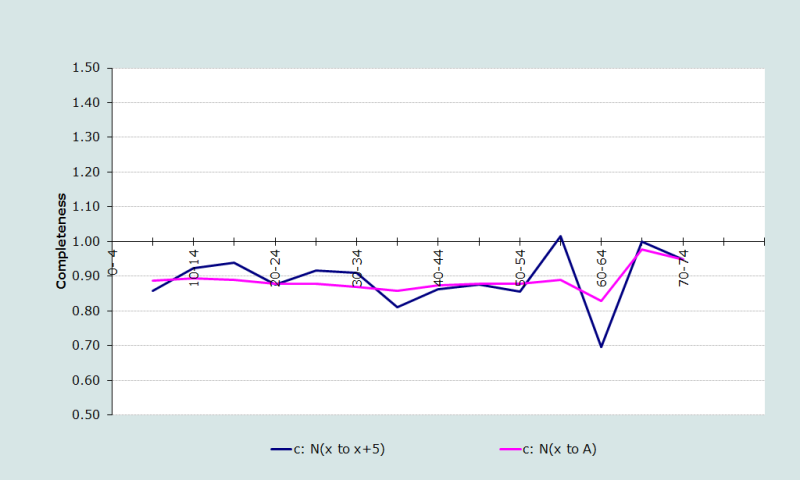
Although the estimate of the growth rate produced by the application of the Brass Growth Balance method produces a satisfactorily level series of ratios, for this example it was decided, for illustrative purposes, to solve for the growth rate and determine the life expectancies iteratively. This produced the plot of ratios shown in Figure 1.

Since there is no consistent trend (either upwards or downwards) apparent in Figure 1 the growth rate was determined using data for ages 5 to 74 by minimizing the deviations from the mean using Solver. Completeness was estimated from the ratios in the age range 15 to 64 to avoid the fluctuations in the estimates for completeness at the oldest ages (although this aspect of determining the estimate is fairly robust to fluctuations at individual ages). This produced an estimate of completeness of 88 per cent as follows:

$$\begin{array}{l}\text{}c=\left(0.5\times 0.8764+0.25\left(0.8575+0.9144\right)\right)\exp \left(0.0306\left(1961.34-1961.50\right)\right)\\ =0.8812\times 0.995=87.7\%\end{array}$$

 

Image

Figure 1 Completeness by age of registered deaths: El Salvador 1961

Step 7: Estimate mortality rates adjusted for incompleteness of reporting of deaths

The population as at the mid-point of the period over which the deaths were recorded is estimated by adjusting the census population for the growth between the two dates at the estimated growth rate of 3.1 per cent. These estimates are shown in the second column of Table 3. For example, for the 15-19 age group the number is estimated as follows:

$${\text{}}_5{N}_{15}(t_m)=125040\times \exp (-0.0306(1961.34-1961.50))=125040e^{0.0306\times 0.16}=125655.7$$

Next, the deaths are adjusted for incompleteness by dividing the number of reported deaths in each age group by the estimate of completeness. These numbers are shown in column 3 of Table 3. For example, for the 15-19 age group the number is derived from the number of reported deaths (shown in column 3 of Table 1), 266, as follows:

$$\text{}\frac{266}{0.8768}=303.4$$

The adjusted person-years of life lived (column 4 of Table 3) are the numbers in the population at the mid-point of the period over which the deaths have been recorded (column 2 Table 3) multiplied by the length (in years) of the period over which the deaths are recorded, which in this case is 1 year.

The mortality rates adjusted for incompleteness of reporting of deaths (column 5 of Table 3) are derived by dividing the adjusted deaths by the adjusted person-years of life lived. For example, for the 15-19 age group the adjusted rate is calculated as follows:

$$\text{}\frac{303.38}{125656}=0.00241\text{}$$

Table 3 Calculation of adjusted mortality rates, El Salvador, 1961 Census

Age	Adjusted 5Nx(tm)	Adjusted 5Dx	Adjusted PYL(x,5)	Adjusted 5mx
0-4
5-9	191,171	696	191,171	0.0036
10-14	150,274	244	150,274	0.0016
15-19	125,656	303	125,656	0.0024
20-24	114,049	332	114,049	0.0029
25-29	92,114	309	92,114	0.0034
30-34	78,094	359	78,094	0.0046
35-39	73,295	398	73,295	0.0054
40-44	57,222	385	57,222	0.0067
45-49	46,433	407	46,433	0.0088
50-54	38,806	439	38,806	0.0113
55-59	26,283	441	26,283	0.0168
60-64	29,417	738	29,417	0.0251
65-69	15,038	512	15,038	0.0341
70-74	11,260	575	11,260	0.0510
75+	16,273	1,551	16,273	0.0953

Step 8: Smooth using relational logit model life table

Estimates of probabilities of women aged x dying in the next 5 years, ₅q_x, estimated from the adjusted rates of mortality are shown in the second column of Table 4. For example, the probability of a 15-year old woman dying before reaching age 20 is calculated as follows:

$${\text{}}_5{q}_{15}=\frac{5\text{}\times 0.00241}{1+2.5\text{}\times 0.00241}=0.0120$$

The life table proportions of five-year olds alive at age x+5 estimated from the proportion alive at age x using these values appear in column 3 of Table 4. For example the proportion alive at age 20 is calculated as follows:

$$\text{}{l}_{20}=0.9740\left(1-\text{}0.01198\right)=0.9623$$

Table 4 Calculation of smoothed mortality rates using a relational logit model life table, El Salvador, 1961 Census

Age	5qx	lx/l5	Obs. Y(x)	Princeton West Cdn. ls(x)	Cdn. Ys(x)	Fitted Y(x)	Fitted l(x)	T(x)	e(x)	Smooth 5mx
0
5	0.0180	1		1			1	61.254	61.3	0.0025
10	0.0081	0.9820	-1.9987	0.9890	-2.2506	-2.1834	0.9875	56.285	57.0	0.0019
15	0.0120	0.9740	-1.8122	0.9805	-1.9585	-1.8980	0.9780	51.371	52.5	0.0028
20	0.0144	0.9623	-1.6204	0.9681	-1.7060	-1.6511	0.9645	46.515	48.2	0.0036
25	0.0166	0.9484	-1.4560	0.9519	-1.4928	-1.4428	0.9471	41.736	44.1	0.0041
30	0.0227	0.9327	-1.3141	0.9337	-1.3226	-1.2765	0.9278	37.049	39.9	0.0047
35	0.0268	0.9115	-1.1658	0.9132	-1.1766	-1.1337	0.9061	32.464	35.8	0.0054
40	0.0331	0.8870	-1.0304	0.8899	-1.0447	-1.0048	0.8818	27.994	31.7	0.0065
45	0.0429	0.8577	-0.8980	0.8628	-0.9194	-0.8824	0.8538	23.655	27.7	0.0081
50	0.0550	0.8209	-0.7611	0.8299	-0.7925	-0.7583	0.8200	19.470	23.7	0.0111
55	0.0806	0.7757	-0.6204	0.7863	-0.6514	-0.6205	0.7757	15.481	20.0	0.0155
60	0.1180	0.7132	-0.4555	0.7289	-0.4946	-0.4672	0.7180	11.747	16.4	0.0235
65	0.1569	0.6290	-0.2640	0.6490	-0.3074	-0.2842	0.6384	8.356	13.1	0.0357
70	0.2263	0.5303	-0.0607	0.5427	-0.0856	-0.0674	0.5337	5.426	10.2	0.0570
75	#N/A	0.4103	0.1814	0.4062	0.1898	0.2018	0.4005	3.090	7.7	0.0903
80	#N/A	#N/A	#N/A	0.2545	0.5373	0.5414	0.2530	1.457	5.8	0.1405
85	#N/A	#N/A	#N/A	0.1201	0.9956	0.9893	0.1215	0.521	4.3	0.2115

The logit transformations of the proportions surviving appear in column 4 of Table 4. For example, the logit transformation of the l₂₀ is calculated as follows:

$${\gamma }_{20}=0.5\ln \left(\frac{1-0.9623}{0.9623}\right)=-1.6204$$

The logit transformation of the conditional life table for females based on the West family of Princeton model life tables with e₀=60 in column 5 of Table 4 appears in column 6 of Table 4. As can be seen from Figure 2 the West model appears to fit the data well, with the possible exception of the youngest ages.

 

Image

Figure 2 Observed logits and adjusted mortality rates against expected derived from the female West model life table, El Salvador, 1961

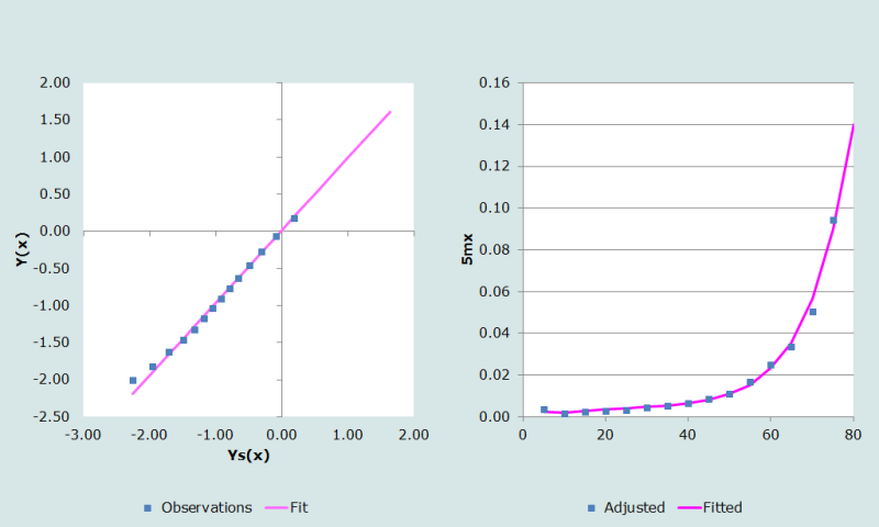
The coefficients, α and β are determined as the intercept and slope of the straight line fitted to the logit transformations in columns 4 and 6 of Table 4 over the range of ages chosen by the user (between 45 and 75 in this example), namely 0.0094 and 0.9754 respectively. The range 45 to 75 is chosen because the fit to the older ages is of importance for estimating the life expectancy at the age of the start of the open interval.

These coefficients are then applied to the logit transformation of the conditional model life table to produce the fitted logits in column 7 of Table 4. Thus, for example the fitted logit at age 20 is calculated as follows:

$${\gamma }_{20}^{fitted}=0.0162+0.9774\times \left(-1.7060\right)=-1.6511$$

These values are then used to produce the fitted life table in column 8 of Table 4. For example the value at age 20 is calculated as follows:

$$l_{20}^{fitted}=\frac{1}{\exp \left(1+2\times \left(-1.6511\right)\right)}=0.9645$$

The conditional years of life lived, T_x, which appear in column 9 of Table 4 are then calculated from the fitted life table. These numbers are used to produce the smoothed mortality rates which appear in column 11 of Table 4. For example, for age 80

$$T_{80}=0.521+\frac{5}{2}\left(0.253+0.1215\right)=1.457$$$${}_5{m}_{80}^{fitted}=\frac{0.253-0.1215}{1.457-0.521}=0.1405$$

The life expectancies which appear in column10 of Table 4 are the numbers in column 9 divided by the numbers in column 8. For example, the life expectancy at age 65 is

$$\text{}\frac{8.356}{0.6384}=13.089\text{}$$

Diagnostics, analysis and interpretation

Checks and validation

The example above was taken from Manual X (UN Population Division 1983) which produced an estimate of completeness of around 83 per cent from applications of both this method and the Brass Growth Balance method. The difference between the two estimates in Manual X and the one produced in this application (89 per cent) appears to be largely due to differences in the method of estimating the population at the age of the open interval (A). The full effect is counteracted to some extent by a reduction (relative to the estimate in Manual X) due to the fact that the current approach solved for a growth rate that was higher (3.02 per cent) than that used in Manual X (2.87 per cent). Thus applying the method using the estimates of life expectancy calculated from the West model life table (column 3, Table 1) produced an estimate of completeness of 85 per cent.

Interpretation

As there is no consistent trend (upward or downward) in the plotted series in Figure 1, there is no reason to reduce the age of the open interval. However, had this been necessary, it would have created a problem in deciding which estimate of completeness to accept, since the estimate of completeness for an open-ended age interval of 70+ is 85 per cent, while that for an interval of 65+ is 76 per cent. The spreadsheet does not allow the open interval to be less than 65+, but, had one used an interval of 60+, the estimate of completeness would have been higher than 76 per cent. As a general rule, it is not recommended in a population with significant digital preference to truncate at an age ending in zero.

Taken together, these estimates suggest that the completeness of death reporting is about 85 per cent, somewhat lower than the 92 per cent estimated by applying the Brass Growth Balance method to these data. Interestingly, had one used the estimates of life expectancy derived from the West life table on the basis of the ratio of ₃₀D₁₀ to ₂₀D₄₀ (and an open interval of 75+) the estimate of completeness drops to 85 per cent but the life expectancy derived from the smoothed rates is closer to that derived iteratively than to those used to produce the estimate of completeness. This suggests that the method is not very sensitive to the estimate of life expectancy used, particularly if the open interval starts at a high age.

Method-specific issues with interpretation

Source of reported deaths

Generally there are two sorts of problems with death data: those that lead to under/over coverage that is constant by age, which is precisely what the method is intended to address, and those which lead to differential coverage by age, which can distort the estimates. Although the general approach remains essentially the same irrespective of the source of the death data, different sources of data are prone to different biases which might impact on the interpretation of the results. These are illustrated by way of particular examples, but, in general terms, you need to look out for the following biases in the death data.

(i)  Vital registration

If the proportionate split of the population between urban and rural (or appropriate proxies) areas differs significantly by age and the completeness of reporting of deaths in urban areas is significantly higher than it is in rural areas, then the assumption that completeness is independent of age is likely to be violated by a falling off of completeness with age at ages over 50 if a proportion of people move from urban to rural areas on retirement. If ignored and the growth rate is estimated using Solver, this violation is likely to lead to an underestimate of the average level of completeness.

(ii) Deaths reported by households in censuses/surveys

The data are subject to three potential problems:

• If a significant proportion of households dissolve on the death of a key person (e.g. the sole breadwinner), then the deaths of such people go unreported, leading to a violation of the assumption that completeness is invariant with age. If a significant proportion of deaths in some age groups are of individuals who do not live in private households (for example, they live in homes for the elderly), the breach of the assumption could be even more severe. However, this is not an issue in most developing countries.
• In situations where young adults leave the home they grew up in to work in urban areas, it is possible that they are regarded as being members of more than one household (or of neither household) and their deaths could be reported more than once (or not at all), again leading to a violation of the assumption of constant reporting of deaths by age. In this case, one can limit the impact by ignoring the data below a specific age in determining completeness.
• Reference period error: Since there is often confusion about the exact period for which deaths are to be reported, in addition to uncertainty about exact dates of death, it is possible for there to be overall under- or over-reporting of deaths. Provided one can assume that this is independent of the age of the deceased, this distortion will be accounted for in the estimate of completeness and is not a problem for estimating mortality rates.

(iii) Deaths recorded in health facilities

Little is known about how well this source of data works. However, it can be expected that completeness would depend on the distribution of health services from which the data have been gathered, and in many developing countries such services are likely to be concentrated in urban areas. So again, if the proportion of the population living in urban rather than rural areas varies with age, then completeness cannot be assumed to be independent of age. It is also possible that certain causes will predominate in facilities, and if these causes are significant and age-related, this could lead to a further violation of the assumption of constant completeness by age.

In all such cases, one should avoid the temptation of adjusting the growth rate to produce a level sequence of the ratios. Instead one should ensure that the estimate of c is determined over a range of ages that excludes those in which death reporting is either exceptionally complete or exceptionally incomplete.

General diagnostic interpretation

In practice the sequences of both $${}_5\widehat{N}{}_x/{}_{5}N{}_x$$ and $${}_A\widehat{N}{}_x/{}_{A}N{}_x$$ are affected by violations of the assumptions. However, part of the power of this technique is that most of the typical violations of assumptions produce fairly distinctive characteristic deviations from the expected horizontal line and in certain circumstances these patterns are interpretable. The following are examples:

(a) Incorrect growth rate: If r is too high the sequences of points fall nearly linearly with increasing age towards the underlying value of completeness and vice versa, as can be concluded from inspection of Equation (1) below. The effect is greater for $${}_5\widehat{N}{}_x/{}_{5}N{}_x$$ than for $${}_A\widehat{N}{}_x/{}_{A}N{}_x$$.

(b) Exaggeration of reported age: Typically, relatives reporting deaths exaggerate the person’s age at death more than living individuals reporting their own ages. This produces rising sequences of points which are imperceptible up to the age at which exaggeration begins, followed by a sharp upward curve thereafter. Again it can be seen from inspection of Equation (1) below in that age exaggeration not only leads to an increase in the number of deaths in the older age categories, but, in addition, transfers within a category lead to those deaths being multiplied by a larger exponential term, although this effect is smaller. Such a pattern would also be produced by rising completeness in death registration with age above a certain age. However, there appears to be no evidence of this in practice (Preston, Coale, Trussell et al. 1980).

(c) Age misstatement in the population estimates and age-specific miscounting: This is exhibited by an erratic sequence of the ratios over the age span. Since $${}_5\widehat{N}{}_x$$ is cumulative in form, it tends to follow the age distribution of the population quite closely. Thus if there are zigzags it is likely that the peaks may be associated with age aversion or under-enumeration in the population and troughs with age heaping or over-enumeration in the population. If these fluctuations are independent of the age, they should not distort the estimate of completeness particularly. Blacker (1988) suggested using age groups 18-22, 23-27, etc. to remove zigzags and showed that for the Brass Growth Balance method this removed bias in the estimate of the slope. However, if these distortions are systematic, e.g. unaccounted for migration below a certain age, it may be better to exclude these points from estimating the completeness.

Generally the effect of overstated ages can be largely removed by beginning the open interval at a sufficiently young age to confine most of the overstatement to the open interval.

In order to distinguish a declining sequence of ratios due to improving mortality from that due to the choice of too high a growth rate, one needs to look to evidence from other sources to determine which the more likely explanation is. If the population has experienced a decline in mortality, the median of the ratios of cumulated populations from 10 to, say, 45 ought still to provide a reasonable estimate of the completeness of death registration. Although this method has a lot to recommend it, and is more robust to departure from stability than the Brass Growth Balance method, it is more sensitive than the latter to certain types of age misreporting. Thus, it will not always be possible to obtain a single robust estimate of the completeness of the death data unless one can confirm the assumptions (particularly the growth assumption) by other means.

Detailed description of method

Mathematical exposition

The Preston and Coale method is a special case of the Synthetic Extinct Generations method, with the growth rate of the population aged x+, r(x+) constant for all ages.

The method arises out of work by Preston and Hill (1980) further developed by Preston, Coale, Trussell et al (1980) and has its origins in the method of extinct generations originally proposed by Vincent (1951). It is based on the idea that the number of persons at a particular age at a point in time must equal the total number of deaths arising from this cohort from that time until the last survivor has died.

In a stable and closed population the relationship is:

$$N_x={\displaystyle \sum _{a=x}^{\varpi }{D}_a{e}^{r(a-x)}}$$

where $$D_a$$ are the deaths at the same point in time as $$N_x$$ since in a stable closed population $$D_{a,t}$$, the deaths aged a which are expected to occur t years from the year for which we have recorded deaths, is equal to $$D_a{e}^{rt}$$.

If instead of $$D_a$$ we know $$D_a^r$$, the recorded number of deaths aged x last birthday, and if we estimate the population aged x, $${\widehat{N}}_x$$, by $${\widehat{N}}_x={\displaystyle \sum _{a=x}^{\varpi }{D}_a^r{e}^{r(a-x)}}$$ then $${\widehat{N}}_x/N_x$$, where $$N_x$$ is the true population at the mid-point of the period over which the deaths have been recorded, gives an indication of the percentage registration for ages x and over, c_x+. If the $$N_x$$ are available at some other point in time, then they can be adjusted for the growth over the period between the two times using the growth rate r. However, if the level of completeness is being estimated in order to calculate mortality rates, the same correction would, in effect, be made to both the numerator and the denominator and thus could be ignored.

There is, however, a problem in computing $${\widehat{N}}_x$$ in practice in that the $$D_a^r$$ are unlikely to be available beyond a certain age (and even if they are, are unlikely to be very accurate) with all reported deaths above that age being grouped together in an open interval, $$D_{A+}^r$$ where A is the lower bound of the age interval. However, various methods have been suggested to deal with this problem. For example, Manual X (UN Population Division 1983, 134) suggests that by assuming that the pattern of mortality fits one of the Coale, Demeny and Vaughan (1983) life tables, $${\widehat{N}}_A$$ can be estimated as follows:

$${\widehat{N}}_A=D_{A+}{e}^{rz(A)}$$

where

$$z(A)=a(A)+b(A)+c(A)e^{\left[D_{45+}/D_{10+}\right]}$$

The coefficients have been tabulated (Table 123, UN Population Division (1983: 134, 134)) and $$\text{}{D}_{45+}/D_{10+}\text{}$$ is estimated by $$\text{}{D}_{45+}^r/D_{10+}^r\text{}.$$.

Alternatively, Bennett and Horiuchi (1984) suggested that the population aged A can be estimated using the following formula:

$${\widehat{N}}_A={\text{}}_{\infty }{D}_A\left(\exp \left(r\times e_A\right)-{\left(r\times e_A\right)}^2/6\right)$$

where the life expectancy is interpolated from the West family of Priceton model life tables on the basis of the ratio of the reported deaths between ages of 10 and 40 to those between ages 40 and 60.

Since $${\widehat{N}}_x$$ can be approximated by $$N_{x+5}{e}^{5r}+{}_{5}D{}_x^r{e}^{2.5r}$$ once $${\widehat{N}}_A$$ has been estimated the $$\hspace{0.25em}{\widehat{N}}_x\hspace{0.25em}$$ can be estimated from the$${}_{5}D{}_x^r.$$

Limitations

The major limitations of the method as described above and provided for in the spreadsheet are that it requires that the population be stable and closed to migration and it should not be applied when these conditions do not apply to any significant extent. By way of example of inappropriate usage, application of this method (data available in the SEG_South Africa_males workbook) to estimate completeness of reporting of deaths in South Africa between the 2001 Census and a census replacement survey in 2007, estimating the population in the middle of the period as that average of the two survey populations, provides an estimate of completeness, using the same age range, of 84 per cent. Increasing the minimum age of the range of the data used to fit the straight line to 35 increases the estimate to 86 per cent, still somewhat lower than the estimate of 94 per cent produced using the Synthetic Extinct Generations method.

This method is more vulnerable to age misreporting than the Brass Growth Balance method. In particular, as mentioned above, the common tendency to exaggerate the age reported at death (relative to that recorded at census) will manifest itself by the plotted points rising noticeably from the age above which the ages have been exaggerated. In such a situation it is better to use the growth rate estimated by the Brass Growth Balance method. In addition the method is also, as demonstrated above, sensitive to the choice of open interval if there is extreme digit preference in the data. This is most likely with census data.

The method is less vulnerable to the effects of destabilisation resulting from a rapid change in mortality (Martin 1980). However, as simulation has shown for the Brass Growth Balance method (Rashad 1978), the bias resulting from a slow steady improvement in mortality (as has been experienced by some developing countries in the absence of epidemics, famine and wars) is quite small.

As far as changes in fertility rates are concerned these tend to have little impact on the performance of the method since they affect mainly the youngest age groups, which have a limited influence on the estimate of completeness. If necessary, these age groups can be excluded from determining the growth rate and estimate of completeness.

Migration is likely to affect the young adult population (mainly between 20 and 35) but to have much less effect on deaths, which occur largely in old age. Unaccounted-for immigration will tend to lower the slope and hence lead to an over-estimate of the extent of death registration and an underestimate of mortality rates. Unaccounted-for emigration will have the opposite effect. Some demographers advocate fitting the straight line to data down to age 5 to limit the effect of unaccounted-for migration, on the assumption that any differences in completeness of reporting of deaths at these younger ages from that of the older ages is unlikely to lead to any major distortions since the mortality is very light between ages 5 and 14. However, it doubtful that this adaptation removes much of the bias.

Alternatively one could confine the fit to points above age 35 to remove the bulk of the effect of migration. However, often the data at the older ages are more suspect making the estimate of completeness less reliable. Although using these adaptations probably produces better estimates than simply ignoring migration, there is, unfortunately, little research into the accuracy of the estimated completeness produced by these adaptations.

Technically, if one had reliable estimates of net migration by age, one could adapt the method by replacing the growth rate r by r – ₅i_x, where ₅i_x is the net in-migration rate for the age group x to x+4 last birthday, in deriving $${\widehat{N}}_x$$. However, in practice, in situations where one has to apply this method one rarely has sufficiently reliable estimates of net migration by age to warrant adapting the method.

Fluctuations in the completeness of death registration with age are likely to introduce curvature in the pattern of points. Consequently, it is one of the strengths of this method that if the points for successive age boundaries fall on a reasonably level line then it is probably reasonable to assume that completeness is constant with respect to age. However, where some but not all the points lie on a straight line one may decide to limit the age range used to determine the estimate of completeness.

Further reading and references

Since this method is a particular case of the more general Synthetic Extinct Generations method, readers are referred to that section for further reading.

 

Bennett NG and S Horiuchi. 1984. "Mortality estimation from registered deaths in less developed countries", Demography 21(2):217-233. doi: https://dx.doi.org/10.2307/2061041

Blacker J. 1988. An Evaluation of the Pakistan Demographic Survey. Karachi: Pakistan Federal Bureau of Statistics.

Coale AJ, P Demeny and B Vaughan. 1983. Regional Model Life Tables and Stable Populations. New York: Academic Press.

Martin LG. 1980. "A modification for use in destabilized populations of Brass's Technique for estimating completeness of death registration", Population Studies 34:381-395. doi: https://dx.doi.org/10.2307/2175194

Preston SH, AJ Coale, J Trussell and M Weinstein. 1980. "Estimating the completeness of reporting of adult deaths in populations that are approximately stable", Population Index 46:179-202. doi: https://dx.doi.org/10.2307/2736122

Preston SH and KH Hill. 1980. "Estimating the completeness of death registration", Population Studies 34:394-366. doi: https://dx.doi.org/10.2307/2175192

Rashad HM. 1978. "The Estimation of Adult Mortality from Defective Registration Data." Unpublished PhD thesis, London: University of London.

UN Population Division. 1983. Manual X: Indirect Techniques for Demographic Estimation. New York: United Nations, Department of Economic and Social Affairs, ST/ESA/SER.A/81. https://www.un.org/development/desa/pd/sites/www.un.org.development.desa.pd/files/files/documents/2020/Jan/un_1983_manual_x_-_indirect_techniques_for_demographic_estimation.pdf

UN Population Division. 2011. World Population Prospects: The 2010 Revision, Volume I: Comprehensive Tables. New York: United Nations, Department of Economic and Social Affairs, ST/ESA/SER.A/313. https://www.un.org/development/desa/pd/sites/www.un.org.development.desa.pd/files/files/documents/2020/Jan/un_2010_world_population_prospects-2010_revision_volume-i_comprehensive-tables.pdf

Vincent P. 1951. “La mortalite des vieillards”, Population 6:182–204. doi: https://dx.doi.org/10.2307/1524149