Direct estimation of child mortality from birth histories

Background

In this section, we focus on the use of data from full birth histories (FBH) or truncated birth histories (TBH). The key characteristics of such data are that for each birth included, the date of birth, survival status and (if dead) age at death are recorded. Analysis of the data typically uses life table approaches. Indirect estimation of child mortality, and estimation of child mortality from survival of a recent birth, are covered in the section on indirect estimation of child mortality and the section about the preceding birth technique.

Data requirements and assumptions

Data required

For each woman of reproductive age (in some settings for cultural reasons information collection is limited to ever-married women):

• the name of each child born alive;
• the month and year of birth of each child;
• the child’s sex (optional);
• Whether the child is still alive; and
• if the child has died, the age at death (age at death in the DHS program is collected in days for deaths that occur in the first 28 days of life, in months for deaths at ages one to 23 months, and in years thereafter).

Important assumptions

• Children still alive and children dead are reported with similar accuracy.
• Dates of birth and ages at death are reported with reasonable accuracy.
• No correlation exists between mortality risks of children and survival rates of mothers (whether as a result of mortality or migration) in the population.

Caveats and warnings

The dangers associated with working with directly-collected data arise from two sources. The first is the risk of survivor bias as only living mothers are asked the detailed birth histories used to generate the data. In situations where it is anticipated that deceased mothers might have had different fertility, or different mortality among their children, from surviving mothers, there is a risk of appreciable bias in the estimates derived. Aspects of survivor bias are discussed in the section on the introduction to child mortality analysis the section on the effects of HIV on child mortality estimation.

The second danger is that if an upper age limit is applied to the women from whom detailed birth history data are collected, truncation bias becomes more significant the further back in time one looks. If an age limit of 49 is applied to the collection of the data, this means that for the period 10 years before the survey, information is only available for women who were then aged up to age 39. Hence, child mortality estimated from such data for earlier time periods will be increasingly based on the experience of younger women. In turn, this might lead to measurement bias, as this truncation results in an over-representation of first births among younger women, meaning that child mortality thus estimated is likely to be increasingly overestimated for earlier time periods. There is some evidence that such over-estimation is counter-balanced by underestimation arising from recall bias (and selective omission of children who have died in periods longer in the past).

Data evaluation and data analysis

Regardless of how data have been collected, or of one’s knowledge of how thoroughly interviewers were trained and supervised, careful review of data quality is an essential first step of any analysis. All data sets contain errors. These can result from many sources, such as an interviewer cutting corners or an interviewee simply not knowing the correct answer to a question. Each section below starts with a description of data evaluation techniques, before progressing to analysis methods. These evaluation techniques examine both internal consistency within a data set, and external consistency with other data sets for the same population. It should be noted in passing that the presence of data errors does not necessarily mean that a data set should not be analyzed; the important thing is to know how large the errors are, and take them into account when interpreting the findings.

The full birth history: data quality assessment

The first step in a thorough data quality assessment is to examine the extent of missing values. In an FBH, values may be missing for a number of reasons. For example, whole households included in the original sampling frame may be missing. Further, eligible women within interviewed households may have no data because the woman could not be interviewed. In addition, individual items within an FBH may be missing because the interviewed woman did not know a child’s birth date, or whether a child was still alive, or (if the child had died) the age at death. The proportions of events potentially affected by these errors need to be examined. Missing items may be imputed during data cleaning, but imputed values should be flagged. The absence of missing values should not be taken as strong evidence of data quality, and may in fact be taken as a warning flag: in some surveys, interviewers and supervisors are trained to avoid missing values, and in such cases data may be more or less made up by the interviewer.

The second step in the data quality assessment is to examine the aggregate results for implausible irregularities. The irregularities most often identified are in sex ratios at birth, in annual distributions of live births, and in ages at death. In the absence of intervention, sex ratios in human populations are generally in the range of 100 to 106 males per 100 females. Sex ratios for birth cohorts outside this range are probably indicative of error. Sex ratios that increase for cohorts born a longer time before the survey are particularly clear indicators of an error, in this case under-reporting of female births that occurred in the distant past.

In the absence of major positive or negative events, births will normally be fairly smoothly distributed by calendar year (in that while seasonality is common, this should not affect the annual numbers. Possible errors can be identified by calculating 'birth ratios', defined as

$$\frac{2B_t}{B_{t-1}+B_{t+1}}$$

where B_t is the number of births reported in a given year, t. 

An error commonly found in DHS data sets has come to be called “birth transference”. DHS surveys collect a substantial amount of additional data about children born since some cut-off date, usually 1 January of the calendar year five years before the survey. It is often the case that births that occurred in that year are reported as occurring in the previous year, presumably to reduce work load. This results in a deficit of births in the year following the cut-off, and a surplus in the year immediately before the cut-off. Birth ratios will highlight this error, since the birth ratio for the year starting with the cut-off will be low, and that for the preceding year will be high. Very often, this birth transference is greater for children who have died than for those who are still alive, so it is good practice to calculate separate ratios for surviving and dead children.

Irregularities in reporting ages at death can similarly be identified by calculating ratios of deaths at some age x to the average number of deaths at ages (x-1) and (x+1). In DHS data sets, there is generally an excess of deaths at age 7 days, to a lesser extent at age 14 days, and at age 12 months.

DHS conveniently publishes these data quality indicators at aggregate (national) level in survey reports (often in Appendix C). Analysts wishing to carry out sub-national analyses will need to calculate indicators themselves.

The data quality indicators described above measure internal plausibility. However, data can be internally plausible and still wrong. Data should also be evaluated by comparison with other surveys for the same population. Cohort comparisons are particularly powerful, for example comparing the average number of children ever borne by women aged 30-34 reported in one survey to the average number borne by women aged 35-39 reported in another survey five years later. Similar comparisons can be made of average numbers of children dead. Sequences of births by single calendar year for overlapping periods can also be compared, though one has to bear in mind that births in the past are increasingly truncated in birth histories limited to women aged 15-49 at the time of the survey.

The full birth history: Calculation of child mortality indicators for birth cohorts

Widely used indicators of child mortality are expressed as probabilities. Thus the Infant Mortality Rate (IMR) is (approximately – as conventionally defined, the IMR is infant deaths in a year divided by births in the year, a value which closely approximates ₁q₀) the probability of dying by exact age 1, ₁q₀, and the Under-five Mortality Rate (U5MR) is the probability of dying by age 5, ₅q₀. Strictly speaking, probabilities are real cohort measures, even though most life tables calculate synthetic cohort measures for specified time periods from age-period mortality rates. Calculating cohort probabilities from FBH data is very straightforward. For example, the cohort IMR for births in the 12 to 23 months before the survey is simply the number of such births that died before the age of 1 divided by the number of births. Similarly, the cohort U5MR for births 5 to 9 years before the survey is the number of such births reported to have died before exact age 5 divided by the number of such births. Figure 1 shows the Lexis diagram representation of the age-cohort probability of dying by age 1 for the cohort born in July 2001 (in green), and the age-period mortality of 5-month olds in calendar year 2002 (the blue rectangle, relating to the example used later in this section).

Image

Figure 1: Lexis diagram representation of age-cohort mortality by age 1 (green) and age-period mortality for 5-month olds (blue)

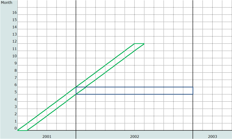
Table 1 shows the relevant numbers and calculations for age-cohort probability of dying by age 1 for the cohort born in the 12-23 months before the survey and for the probability of dying by age 5 for the cohort born in the 5 to 9 years before the survey, using data from the 2004 Malawi DHS. Note that there is no period interpretation of such cohort values; in the U5MR example, the cohort probability reflects mortality risks in every one of the 10 years before the survey. Also note that the probability of dying by age x can only be calculated for cohorts that were born at least x years before the survey. Both these considerations limit the value of the cohort measures, since for most purposes analysts and policy-makers are more interested in time period measures.

Table 1: Calculation of IMR and U5MR for cohorts: Malawi 2004 DHS

The full birth history: Calculation of child mortality indicators for time periods

Period-specific measures are estimated using the synthetic cohort concept. Mortality rates for narrow age ranges and defined calendar periods are calculated on the basis of events and exposure in these rectangles in the Lexis Diagram. The rates are then converted into implied probabilities, using standard demographic relations (see, for example, Preston, Heuveline and Guillot (2001)) and making generally mild assumptions about the distribution of deaths in each rectangle. Finally, the probabilities of dying are applied successively to an initial hypothetical cohort of births to compute a survivorship curve ℓ(x) for each age x, from which it is easy to derive probabilities of dying.

FBH data lend themselves to these life table calculations quite easily. If data are collected following the standard DHS practice – as month and year of birth and age at death in days, months or years, depending on the age – deaths  can be located with little ambiguity in age-period rectangles of the Lexis Diagram. (There will be some residual ambiguity, because of the imprecision of the information on date of birth and age at death, but the impact will depend on the sizes of the rectangles.) Here we describe an approach based on the calculation of age-specific mortality rates for a single calendar year (age-period rates) for mortality up to age 5. Extension to other time periods is straightforward. It is assumed that data are in standard DHS format, that is, birth dates are recorded in century month (CMC) format, and ages at death in days, months or years. Unit record data must be available. The unit of age used is the month. The basic calculations are therefore of age-specific mortality rates by month of age and calendar year. These rates are converted into corresponding probabilities of dying in each month. These probabilities are then converted into probabilities of surviving, and are chained together over whatever age range is required (typically up to age 5). The key to the calculation is to assign deaths and exposure time to one-month age segments across a calendar year.

Data manipulation

Four variables in a DHS birth data set are required:

1. b3, date of birth in CMC;
2. b5, whether child is still alive;
3. b6, age at death, where the first digit represents the unit (1 indicating days; 2, months; and 3, years) and the second and third digits represent the value given that unit; and
4. v005, sample weight, expressed in millions.

Note that variable b7, age at death (months-imputed) is not used. This variable does not lend itself to the mortality rate approach described here, because in cases in which age at death is recorded in years, the 'imputed' month is actually the lower bound of the age interval; that it, if age at death is recorded as '3 years', the imputed age at death in months is recorded as 36 months. Using this variable will result in systematic mis-location of deaths in time.

Application of method

Step 1: Manipulation of age at death and calculation of estimated birth date and age at death

We want to locate deaths in a calendar month of occurrence. Since we do not have a precise date of birth (only CMC), and in general we do not have a precise age at death (except for neonatal deaths), we need to impute both a date of birth and an age at death. We can perform this imputation using random numbers.

It is evidently undesirable – for reasons of lack of reproducibility, amongst others – to make use of a true random number generator to produce the random numbers referred to above. In addition, ‘true’ randomization risks creating a spurious impression of precision. As an alternative, we propose creating pseudo-random numbers from variables that are routinely available in DHS data and that can be applied in the algorithm above. It is an easy matter to create new variables apportioning the records into deciles based on the reported day of interview (v016 in a DHS) and household number (v002). (These variables have been chosen on the grounds that there is unlikely to be any correlation between them and child mortality). These new variables will take the values in the range (0, 1 … 9). Dividing each by 10, and adding 0.05 results in two new uniformly distributed variables, random1 and random2, taking values in the range (0.05, 0.15, … , 0.95). 

It is then straightforward to impute a date of birth (dob, in months) if births in the month of interview are excluded from analysis by adding random1 to b3 (the CMC of the child’s date of birth). The method for imputing an age at death (in units of months) depends on the ‘unit’. For ‘unit’ = 1 (i.e. age at death measured in days), age at death (aad) can be estimated as (‘value’+ random2)/31 (for age at death in days this is not necessary, but is described for symmetry); for ‘unit’ = 2, age at death is ‘value’ + random2; and for ‘unit’ = 3, age at death is (‘value’ + random2)*12.

Step 2: Location of deaths in target year

For each month-of-age mortality rate, the events consist of deaths at that age in the period of investigation. Step 1 has imputed age at death in months. The date of death dod is given by the sum of imputed month of birth dob and imputed age of death aad. If imputed age at death is within the age range and the imputed date of death falls within the period of investigation, we have a relevant event.

Step 3: Derivation of exposure to risk

The calculation of exposure to risk is intricate, but relatively straightforward. The age range of the investigation refers to those ages (defined in appropriate units) for which we want to measure mortality. We define the lower bound of the age range to be x_l, and the upper bound to be x_u.

The period of investigation is the measure of the time period for which we seek to estimate mortality, and is defined as the period (t₂ - t₁), where t₂ is the end date of the period of investigation, and t₁ the start date, measured in the same units as that defined by the age range.

Graphically, then, we seek to measure mortality in the age and period defined by the heavy lines in Figure 2.

Image

Figure 2: Lexis diagram showing calculation of exposure to risk

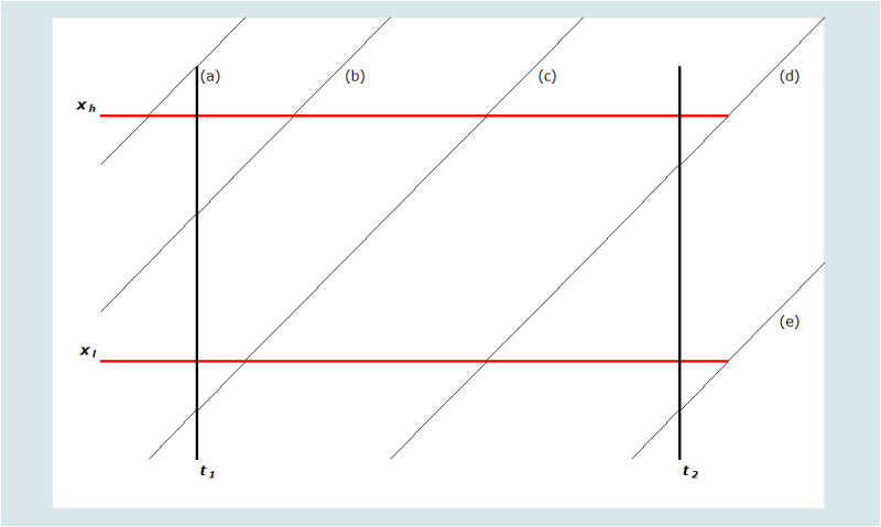
An individual’s life course by age and period is represented by the diagonal lines (as with a conventional Lexis diagram). Five possible scenarios (labelled (a) through (e)) are portrayed. Any individual’s position in the space can be defined by their age at t₁, x_t1. It follows, further, that any person aged x at t₁, if she or he does not die before t₂, would be aged x_t2 = x_t1 +(t₂ - t₁) at time t₂. We define the age at death of those deaths that occur in the specified age range in the period of investigation to be x_d. The relative contribution of each scenario to the exposure to risk is determined by the algorithms in Table 2.

Table 2: Algorithm for determining exposure to risk

Applying these rules to define the exposure in the age range in the period of investigation for each individual and aggregating gives the total exposure to risk, which is the denominator for the mortality rate. Summing the deaths occurring in the age range in the period of investigation provides the numerator.

Step 4: Weighting and cumulating events and exposure time

The sample weight variable in a standard DHS recode file is v005. This variable has a mean of 1,000,000. To avoid the appearance of huge sample sizes (and much too narrow confidence intervals) it is recommended first to recalculate the weight as (v005/1,000,000). Let us call this new variable wgt. Mortality rates can be calculated by considering the contributions of each of the N children in the survey to the number of events and the total exposure time. The age-specific mortality rate age x to x + 1 (in months) in a period, j, is

$$M\left(x,j\right)=\frac{{\displaystyle \sum _{i=1}^{N}D\left(i,x,j\right).wgt\left(i\right)}}{{\displaystyle \sum _{i=1}^{N}E\left(i,x,j\right).wgt\left(i\right)}}$$

where M(x,j) is the age specific rate for age x and year j, D(i,x,j) is a binary variable indicating the death of child i at age x in year j (1 if the death occurs, 0 otherwise), E(i,x,j) is the exposure time of child i at age x in year j, and wgt(i) is the sample weight (mean 1.0) of child i.

Step 5: Calculating probabilities of dying from age-specific mortality rates

The rates calculated in Step 4 are per month of age exposure. It is therefore necessary to adapt the standard formula for deriving a period probability of dying from a rate to take this into account. Given that we have made a number of simplifying assumptions and are working with narrow age ranges, it is adequate to assume that deaths are evenly distributed across each single month age range. We can then calculate q(x) as

$$q\left(x,j\right)=\frac{\frac{M\left(x,j\right)}{12}}{\left(1+\frac{M\left(x,j\right)}{24}\right)}$$

Survivorship probabilities from birth to any age can then be obtained by chaining together survivorship by month (i.e. (1-q(x,j)) ) terms. Thus for instance

$${}_{5}q{}_{{}_0}^j=1-{\displaystyle \prod _{x=0}^{59}\left(1-q\left(x,j\right)\right)}$$

Worked example

As noted above, direct estimation of child mortality from a birth history requires working with unit record data rather than tabulations. As a worked example, we will therefore illustrate with a limited number of records adapted from a DHS, specifically the mortality of 5-month olds in 2002 from the 2004 Malawi DHS. Only children born between 1 July 2001 and 31 July 2002 are at risk of dying at age 5 months in calendar year 2002 (children born before 1 July 2001 would be aged 6 months or more by the beginning of calendar year 2002, and those born after 31 July 2002 would not have reached age 5 months in the year). Only relevant records are shown, that is, those for births between month 1218 and 1230 in CMC terms (July 2001 to July 2002). In practice, we would also exclude any births that died before five months of age, but we will include them in the example to show that we exclude them from calculations.

Table 3 shows the key variables for 50 records from the 2004 Malawi DHS; note that these are birth records, not woman records.

Table 3: Basic birth history data for direct estimation of child mortality

Step 1: Manipulation of age at death and calculation of estimated birth date and age at death

Random numbers random1 and random2 are derived as described above, resulting in revised values of dates of birth and age at death, dob' and aad'. The date of death dod' is estimated as the sum of the imputed month of birth dob' and imputed month of death aad'. Column 10 of Table 4 shows dod'.

Table 4: Derivation of imputed date of birth, age at death and date of death, Malawi, 2004 DHS (50 cases)

Step 2: Location of deaths in target year

A relevant death in terms of period is one with a CMC between 1224 to 1235. The deaths in records 3, 6, 31 and 41 of Table 4 are therefore not relevant because they are deemed not to have occurred in 2002. The deaths in records 11 and 45 are not relevant because the child died at 2 months (11) or 1 month (45) of age, and therefore was not exposed to the risk of dying at age 5 months.

Step 3: Derivation of exposure to risk

Table 5 presents the calculation of the exposure to risk for the 50 cases described above. The rule used to determine the exposure is presented in the column headed ‘Scenario’. The resulting exposure is presented in the following two columns for those who survive the period of investigation and those that die during the period.

For children who survive to age 6 months, those born in months 1219 to 1229 contribute a full month of exposure time to the age-period of interest (i.e. from exactly 5 to exactly 6 months). Thus record 1 (born 1223.55) contributes a full month. A child born in month 1218 will contribute (dob - 1218) months, so record 23 (born 1218.85) contributes 0.85 of a month; and a child born in month 1230 will contribute (1231 - dob) months, so record 7 contributes 1231 - 1230.55 = 0.45 months. The children born in months 1219 to 1229 who die at age 5 months will contribute (aad - 5) months of exposure; thus the death in record 14 occurs at 5.25 months and contributes 0.25 months of exposure.

Table 5: Derivation of exposure to risk for estimation of child mortality, Malawi, 2004 DHS (50 cases)

Step 4: Weighting and cumulating events and exposure time

The final step before calculating the death rate is to take account of the record sample weight in both the deaths and the exposure time, and then sum the weighted deaths and exposure. Columns 6 and 7 of Table 5 show the exposure to risk for survivors and relevant deaths. Columns 8 and 9 then multiply columns 6 and 7 respectively by the sample weight v005/1,000,000. The age-specific mortality rate M(5,2002) is then calculated by dividing the sum of the weighted deaths by the sum of the weighted exposure time:

$$M\left(x,j\right)=\frac{{\displaystyle \sum _{i=1}^{N}D\left(i,x,j\right)*wgt\left(i\right)}}{{\displaystyle \sum _{i=1}^{N}E\left(i,x,j\right)*wgt\left(i\right)}}=\frac{6.389}{59.317}=0.1077$$

Step 5: Calculating probabilities of dying from age-specific mortality rates

The rates calculated in Step 4 are per month of exposure. It is therefore necessary to adapt the standard formula for deriving a period probability of dying from a rate. Given that we have made a number of simplifying assumptions and are working with narrow age ranges, it is adequate to assume that deaths are evenly distributed across each single month age range, even for the first month of life. We can then calculate q(x) as

$$q\left(5,2002\right)=\frac{\frac{M\left(5,2002\right)}{12}}{\left(1+\frac{M\left(5,2002\right)}{24}\right)}=\frac{\frac{0.1077}{12}}{\left(1+\frac{0.1077}{24}\right)}=\frac{.008975}{1+0.004488}=0.008935$$

Once all the q(x,j)s have been calculated, they can be converted into their complements, probabilities of surviving, and chained together to produce survivorship probabilities and probabilities of dying from birth to any desired age.

To obtain rates and probabilities for periods longer than a single calendar year, the weighted sums obtained in Step 4 are summed across years as required. Step 5 remains exactly the same.

Note that the procedure described here differs from that used by DHS. The DHS approach calculates probabilities directly for quasi-cohorts (Croft et al. 2023). Calculations are made for eight age groups: neonatal, 1-2 months, 3-5 months, 6-11 months, and years from age 1 to age 4. For each age range, period deaths are derived from date of birth and age at death. The risk set is an approximation of the number of children who enter that age range during the period. This approximation is the sum of all children who enter the age range and leave the age range (or would do so if they survived) during the time period, plus half of those who enter the age range during the period but would leave it after the period, plus half of those who enter the age range before the period but would leave it during the period.

Whichever procedure is used, individual-level data from the FBH will be required. Although the calculations could be carried out from detailed tables, it would be very tedious to do so. Use of a suitable computer routine is strongly recommended.

Interpretation

The key characteristic of direct child mortality estimation, namely that information is provided by surviving women who still live in surveyed households, needs to be borne in mind when interpreting results as there is risk of respondent selection bias. In particular, the mortality experience of children born in a community whose mothers no longer live in the community will not be included in the measures. If such children have higher mortality than those born to mothers who do still live in the community, mortality will be under-estimated. The most severe form of this bias is likely to result from substantial levels of HIV prevalence in the community, since such prevalence in the absence of widespread antiretroviral therapy will result in a strong positive correlation between survival of child and survival of mother (see effects of HIV/AIDS on child mortality estimation). However, some positive correlation between mother and child survival is almost certain in any population. Other reasons for bias may exist. For example, high in-migration rates will result in women reporting on the survival of children born and raised elsewhere, while high out-migration will remove responses about children who were born and raised in the community. Although it is impossible to know a priori the direction or magnitude of such biases, the analyst needs to keep in mind their potential effect. Non-response may also be an issue if women absent from the community for an extended period cannot be interviewed in person, but may have experienced different risks to their children, or may not be present in part because their children have experienced different risks.

Extension to the method: Truncated birth histories

Truncated birth history: Data quality assessment

The truncated birth history (TBH) provides fewer opportunities for data quality checks than the full birth history (FBH) because the time series of events reported is by definition truncated. If the truncation is by time period, the events reported should be representative of the time period covered, whereas if the truncation is by number of events, the events reported may be representative only of all events in quite a short period prior to the survey, and this will complicate any assessment of the sequence of events in time.

As with the full birth history, the first step should be to examine the data for missing values. The second step should involve the examination of sex ratios at birth and heaping on ages at death.

No direct assessment of birth transference will be possible, because no detailed information about dates of births is available prior to the truncation point. However, an indirect assessment is possible. A TBH should always involve the initial collection of a summary birth history. The births and child deaths for an age group of women defined as at the survey date can therefore be calculated both at the time of the survey (from the summary birth history) and (only approximately for the deaths) at the truncation point, by subtracting the births and child deaths reported in the TBH. The calculation for births is precise, but for child deaths is approximate because some of the child deaths reported in the summary birth history (SBH) will have occurred during the post-truncation period to children born before the truncation point; typically, however, the number of such extra deaths will be small given that child mortality risks drop rapidly with age of child. The data quality assessment is therefore the comparison of the proportion dead (by age group of mother at the time of the survey) of the children born after the cut-off date to that of the children born before the cut-off date.

There are two reasons why the former proportion will generally be smaller than the latter. First, the children will have been exposed to the risk of dying for a shorter period. Second, if child mortality is falling over time, they will have been exposed to lower age-specific risks as well. However, if children who have died are systematically omitted from the post-truncation period, or if they are reported in the summary birth history but not reported as having been born in the period, the ratio of the two will be inflated by data error. We can estimate a plausible error-free ratio if data are available from a full birth history for the same population at an earlier or later date. Table 6 shows data from Mongolia: three Reproductive Health Surveys, one in 1998 that included a full birth history and two – one in 2003 and one in 2008 – that collected only TBHs. The 1998 full birth history data are used to calculate proportions dead for children born before and after a comparably-defined cut-off date, and compared to the proportions calculated from the 2003 and 2008 TBH data. As can be seen, the TBH ratios are several times larger than the full birth history ratios, providing compelling evidence of transference of dead children out of the post-truncation period. In the absence of a country-specific baseline, such as that provided here by the 1998 RHS survey, ratios of 3 or higher should be taken as evidence of probable omission of dead children from the recent reference period.

Table 6: Proportions of children dead by whether the birth occurred before or during the TBH date window, Mongolia, 1998, 2003 and 2008 RHS

The truncated birth history: Calculation of child mortality indicators for cohorts

The calculation of cohort probabilities of dying from a TBH follows the same principle as that followed with a FBH: the probability of dying by age x is calculated as the number of dead children to the number of children ever born in some defined cohort born no less than x years before the survey. There is an important difference, however, as made clear in the Lexis Diagram in Figure 1, namely that the value of x is constrained by the truncation date. For example, if the truncation date is 5 years before the survey, no birth cohort will have been fully exposed to the full risk of dying by age 5, and the cohorts exposed fully to risks up to age 2 are limited to births 2, 3 and 4 years before the survey. Thus there are limits to the range of ages for which mortality indicators can be derived.

The truncated birth history: Calculation of child mortality indicators for time periods

The basic approach to calculating standard indicators from a TBH follows the same principles as that used for a full birth history: to calculate age-specific rates for a specified time period, convert them into estimates of probabilities of dying in successive age intervals, and apply the probabilities to a synthetic cohort of births to create the life table. The problem with analyzing a TBH in this way is the same, however, as that faced in calculating cohort indicators, namely that cases and exposure time become progressively more restricted as age increases. Thus if the cut-off point is five years before the survey, the measures for ages 3 and 4 will be based on small numbers and have wide sampling errors.

References

Croft, Trevor N., Allen, Courtney K., Zachary, Blake W., et al. 2023. Guide to DHS Statistics. Rockville, Maryland, USA: ICF. https://www.dhsprogram.com/Data/Guide-to-DHS-Statistics/index.cfm

Preston SH, P Heuveline and M Guillot. 2001. Demography: Measuring and Modelling Population Processes. Oxford: Blackwell.