The Brass Growth Balance Method
Description of method
Brass’s Growth Balance method (Brass 1975) is the first of what later became known as the Death Distribution Methods for estimating the completeness of the reporting of deaths relative to an estimate of the population. The method makes use of the observation that in a stable population (i.e. a population with an unchanging age structure over time – at least for the adult ages – growing at a constant rate, r, each year) that is closed to migration and has accurately reported data, the growth rate, r, is equal to the birth rate, b, less the death rate, d. A similar relationship holds for the population aged x and older, namely, that , where the partial "birth" rate, , is defined as the rate at which people turn age x in the population aged x and older and the partial death rate, , is the rate of mortality of people aged x and older. If, in this population, the deaths are under-reported to the same extent at each age, then , where is the death rate based on the recorded deaths for ages x and older and c is the proportion of deaths that are reported. One can estimate c from the slope of a line fitted to the , data points. This estimation is usually confined to adult ages as the (extent of) completeness of reporting of child deaths usually differs from that of adult deaths. Mortality rates can be estimated by dividing the numbers of deaths reported in each age group by c and then dividing these numbers by an estimate of the population exposed to risk based on the population used to estimate the partial birth and death rates.
The method is a particular case of the more general Generalized Growth Balance method, which requires estimates of the population at two points in time but does not require that the population be stable. Readers are referred to that section for further detail on the method. It is included in this manual as a method that might be considered when one has an estimate of population numbers only at one point in time.
Data requirements and assumptions
Tabulations of data required
- Number of deaths of women (men), by five-year age group, and for open age interval A+ (with A as high as possible), over a specific period.
- Number of women (men), by five-year age group, and for open age interval A+, at or close to the period over which the deaths were measured.
Important assumptions
- The population is stable, although this assumption can be relaxed to some extent (see below).
- That the completeness of reporting of deaths is the same for all ages above a minimum age (usually age 15)
- The population is closed to migration, although this assumption can be relaxed if net migration is small relative to the mortality rates, or if one has reasonably accurate estimates of the number of migrants by age to allow for in the balance equation (which is very seldom the case).
Preparatory work and preliminary investigations
Before applying this method, you should investigate the quality of data at least in the following dimensions:
- age structure of the population;
- sex structure of the population;
- age structure of deaths; and
- sex structure of the deaths.
Caveats and warnings
In applying this method, analysts must take particular care with the following:
- The interpretation and estimation processes need to take into account the source (whether vital registration, deaths reported by households in censuses, or deaths recorded at health facilities) of death data as explained below. However, the biases associated with the source of death data tend to have less impact on the estimate of completeness from the Growth Balance method than on that from the Synthetic Extinct Generations method.
- If applying the method to sub-national geographic areas, the issue of migration typically becomes a greater concern.
- Deciding the age range which is used to fit the straight line to the partial birth and death rates and hence estimate completeness. Issues here are the best age to choose for the open interval if there is evidence of age exaggeration; how to accommodate data points that rise above the line at the older ages because of decreasing completeness with age, possibly due to retirement-associated migration from urban to rural areas where registration is less complete; and whether to exclude ages less than either 30 or 35 because of the impact of migration which has not been allowed for specifically.
- If completeness of reporting of deaths appears to be less than 60 per cent then caution is advised in applying this method as the uncertainty about the estimate is large.
Application of the method
Step 1: Cumulate population and deaths downwards
To estimate partial birth and death rates one needs to cumulate the numbers in the population and the number of deaths in a defined period of t years for ages x and older. In the case of the population the following equation is used:
where A is the age at the start of the open age interval.
An analogous equation is used to calculate the number of deaths aged x and older, D(x+).
Step 2: Calculate the person-years of life lived, PYL(x+)
In order to estimate partial birth and death rates one needs to estimate the person-years of exposure. This is estimated using the following formula:
where t is the length of period over which the deaths have been measured.
Step 3: Calculate the number of people who turned x in the population, N(x)
The number of people who turned x (i.e. were ‘born’ into the open age interval x+) in the population is estimated as the geometric mean of the numbers in the two adjacent (five-year) age groups divided by 5, multiplied by the length of the period over which the deaths are reported, in years, using the following formula:
Step 4: Calculate partial ‘birth’ and death rates, b(x+) and d(x+)
The partial birth and death rates are estimated using the following formulae:
and
respectively.
Step 5: Plot graph, fit line and estimate completeness, c
In order to estimate the completeness of reporting of deaths relative to the population, one starts by plotting b(x+) against d(x+) and estimating the coefficients of the straight line fitted to these points, using orthogonal regression, as follows:
and
where b is the slope of the line and a the intercept, and yi represent the b(x+) and the xi represent the d(x+) and and represent the means of the two series, respectively.
After fitting the straight line to all the points, one inspects the plotted points relative to the line and the residuals in order to decide on the best range of ages to use to determine the completeness of reporting of deaths. How one decides this is discussed in more detail below, but any points with residuals greater than 1 per cent in absolute value should be excluded. A line is then fitted to the remaining points, and new values of a and b are determined from the fitted line.
The completeness of reporting of deaths, c, is derived from these values of a and b as follows:
where tc is the time of the census and tm is the mid-point of the period over which the deaths have been recorded. The rationale for this equation is that the reciprocal of the slope estimates the completeness of reporting on the assumption that the census population was at the mid-point of the period over which the deaths have been recorded. In order to correct for any difference between the time of the census and the mid-point of the period over which the deaths have been recorded we need to multiply the estimate of completeness by the ratio of the census population to the estimate of the population at time tm. This is done on the assumption that the population, which is assumed to be stable, is growing at an annual growth rate estimated by a. That ratio is .
Step 6: Estimate mortality rates adjusted for incompleteness of reporting of deaths
In order to compute mortality rates one needs first to estimate the population in five-year age groups at the mid-point of the period over which the deaths were recorded by multiplying the census numbers by .
Next one needs to adjust the number of deaths for incompleteness by dividing the reported number of deaths by the estimate of completeness, c.
The person-years of exposure are estimated by multiplying the estimated population as at tm by the length of the period over which the deaths were reported, t.
Mortality rates adjusted for the incompleteness of the reporting of deaths are thus estimated as follows:
Since both the numerator (through the estimate of c) and the denominator are adjusted by , omitting these adjustments would still produce the same estimates of mortality rates. The estimate of completeness, however, would be equivalent to what it would be if the population at tm was that at tc.
Step 7: Smooth using relational logit model life table
Because the age-specific rates can be erratic they need to be graduated (smoothed). This can be achieved by fitting a Brass relational logit function to a sex-specific standard life table which is considered to have the same shape as that generated by the mortality rates of the population being investigated.
The accompanying workbook contains a spreadsheet that allows one to produce a smooth set of mortality rates by using a relational logit model fitted to the life table generated by the adjusted mortality rates. The user can choose a standard from the General family of United Nations model life tables or from any of the four families of Princeton model life tables. Other life tables can be used as standard if there is reason to assume that they it better resembles the pattern of adult mortality in the population being studied.
In order to fit the model, probabilities of people aged x dying in the next 5 years, 5qx, are estimated from the adjusted rates of mortality as follows:
From this the life table with a radix of l5 = 1 is calculated as follows:
The coefficients, α and β are determined by fitting the relational logit model as follows:
where
and superscript ‘s’ designates values based on a standard life table.
The fitted life table is then generated from the standard life table using the coefficients α and β as follows:
and
The smoothed mortality rates are derived from this life table as follows:
and
where
i.e.
and ω is the age above which the life table has no more survivors.
Worked example
This example uses data on the numbers of women in the population from the El Salvadorian Census in 1961 and on deaths from vital registration for the calendar year 1961. The example appears in the BGB_El Salvador workbook. The reference date for the 1961 Census was midnight between 5 and 6 May, so the date of the census is entered as 1961/05/06 on the Introduction sheet.
Step 1: Cumulate population, deaths and migrants downwards
One accumulates the numbers in the population and deaths from the oldest age downwards (Table 1).
Table 1 Calculation of the cumulated population and deaths, El Salvador, 1961 Census
Age | 5Nx | 5Dx | N(x+) | D(x+) |
|---|---|---|---|---|
0-4 | 214,089 | 6,909 | 1,274,253 | 13,652 |
5-9 | 190,234 | 610 | 1,060,164 | 6,743 |
10-14 | 149,538 | 214 | 869,930 | 6,133 |
15-19 | 125,040 | 266 | 720,392 | 5,919 |
20-24 | 113,490 | 291 | 595,352 | 5,653 |
25-29 | 91,663 | 271 | 481,862 | 5,362 |
30-34 | 77,711 | 315 | 390,199 | 5,091 |
35-39 | 72,936 | 349 | 312,488 | 4,776 |
40-44 | 56,942 | 338 | 239,552 | 4,427 |
45-49 | 46,205 | 357 | 182,610 | 4,089 |
50-54 | 38,616 | 385 | 136,405 | 3,732 |
55-59 | 26,154 | 387 | 97,789 | 3,347 |
60-64 | 29,273 | 647 | 71,635 | 2,960 |
65-69 | 14,964 | 449 | 42,362 | 2,313 |
70-74 | 11,205 | 504 | 27,398 | 1,864 |
75+ | 16,193 | 1,360 | 16,193 | 1,360 |
Step 2: Calculate the person-years of life lived, PYL(x+)
As the deaths are recorded over a single year, the person-years of life lived (column 2 of Table 2) are simply the cumulated numbers in the census (i.e. the same as column 4 of Table 1) as multiplying by one leaves the numbers unchanged.
Table 2 Calculation of the person-years lived, the number reaching age x, partial birth and death rates and residuals, El Salvador, 1961 Census
Age | PYL(x+) | N(x) | b(x+) | d(x+) = X | b(x+) = Y | a+bx | Residuals y-(a+bx) |
|---|---|---|---|---|---|---|---|
0-4 | 1,274,253 |
|
| 0.00000 |
| 0.03097 |
|
5-9 | 1,060,164 | 40,362 | 0.03807 | 0.00636 | 0.03807 | 0.03782 | 0.00026 |
10-14 | 869,930 | 33,733 | 0.03878 | 0.00705 | 0.03878 | 0.03856 | 0.00022 |
15-19 | 720,392 | 27,348 | 0.03796 | 0.00822 | 0.03796 | 0.03981 | -0.00185 |
20-24 | 595,352 | 23,825 | 0.04002 | 0.00950 | 0.04002 | 0.04119 | -0.00117 |
25-29 | 481,862 | 20,399 | 0.04233 | 0.01113 | 0.04233 | 0.04294 | -0.00061 |
30-34 | 390,199 | 16,880 | 0.04326 | 0.01305 | 0.04326 | 0.04501 | -0.00175 |
35-39 | 312,488 | 15,057 | 0.04818 | 0.01528 | 0.04818 | 0.04741 | 0.00077 |
40-44 | 239,552 | 12,889 | 0.05380 | 0.01848 | 0.05380 | 0.05085 | 0.00295 |
45-49 | 182,610 | 10,259 | 0.05618 | 0.02239 | 0.05618 | 0.05506 | 0.00112 |
50-54 | 136,405 | 8,448 | 0.06193 | 0.02736 | 0.06193 | 0.06040 | 0.00153 |
55-59 | 97,789 | 6,356 | 0.06500 | 0.03423 | 0.06500 | 0.06779 | -0.00279 |
60-64 | 71,635 | 5,534 | 0.07725 | 0.04132 | 0.07725 | 0.07542 | 0.00183 |
65-69 | 42,362 | 4,186 | 0.09881 | 0.05460 | 0.09881 | 0.08970 | 0.00911 |
70-74 | 27,398 | 2,590 | 0.09452 | 0.06803 | 0.09452 | 0.10415 | -0.00963 |
75+ | 16,193 |
|
|
|
|
|
|
Step 3: Calculate the number of people who turned x in the population, N(x)
The numbers of people who turned x are shown in the third column of Table 2. For example, the number who turned 70 is estimated as follows:
Step 4: Calculate partial birth and death rates, b(x+) and d(x+)
The partial birth and death rates are given in the fourth and fifth columns of Table 2. For example these are, for age 20:
and
Step 5: Plot graph, fit line and estimate completeness, c
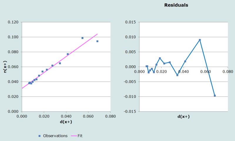
In order to plot the graph and fit the line to all of the data points, one starts by setting the lower age to 5 and the upper age to A-1, where A represents the age at the start of the open age interval (75 in this example). The plotted values of b(x+) against d(x+) are shown in Figure 1 and the coefficients of the straight line fitted to these points are estimated as follows:
Inspection of the diagnostic plots in Figure 1 suggests that all but the last (most right-hand) two points lie acceptably close to the fitted line with little evidence of significant migration. Although the residuals of the last two points fall just within the 1 per cent tolerance limits and one could use the estimate of completeness of 93 per cent, it is a useful check to consider the estimate if those two points were dropped.
The completeness of reporting of deaths, c, is derived from these values of a and b as follows:
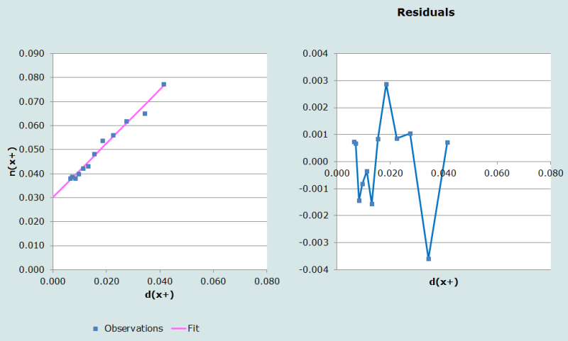
Dropping the last two points (by setting the upper age of the chosen range to 64) produces the diagnostic plots shown in Figure 2 and an estimate of completeness of 89 per cent, which is sufficiently close to suggest that it is unnecessary to drop the last two points. Dropping only the last point produces a big change in the estimate (to 82 per cent) and a poorer fit for some of the points to the left, which suggests that this is probably not the best course of action. As a general rule, it is not recommended in a population with significant digital preference to truncate at an age ending in zero.
Step 6: Estimate mortality rates adjusted for incompleteness of reporting of deaths
The population as at the mid-point of the period over which the deaths were recorded is estimated by adjusting the census population for the growth between the two dates at the estimated growth rate of 3.1 per cent. These estimates are shown in the second column of Table 3. For example for the 15-19 age group the number is estimated as follows:
Next the deaths are adjusted for incompleteness by dividing the number of reported deaths in each age group by the estimate of completeness. These numbers are shown in column 3 of Table 3. For example, for the 15-19 age group the number is derived from the number of reported deaths (shown in column 3 of Table 1), 266, as follows:
The adjusted person-years of life lived (column 4 of Table 3) are the numbers in the population at the mid-point of the period over which the deaths have been recorded (column 2 Table 3) multiplied by the length (in years) of the period over which the deaths are recorded, which in this case is 1 year.
The mortality rates adjusted for incompleteness of reporting of deaths (column 5 of Table 3) are derived by dividing the adjusted deaths by the adjusted person-years of life lived. For example, for the 15-19 age group the adjusted rate is calculated as follows:
Table 3 Calculation of adjusted mortality rates, El Salvador, 1961 Census
Age | Adjusted 5Nx(tm) | Adjusted 5Dx | Adjusted PYL(x,5) | Adjusted 5mx |
|---|---|---|---|---|
0-4 |
|
|
|
|
5-9 | 191,181 | 659 | 191,181 | 0.0034 |
10-14 | 150,282 | 231 | 150,282 | 0.0015 |
15-19 | 125,662 | 288 | 125,662 | 0.0023 |
20-24 | 114,055 | 315 | 114,055 | 0.0028 |
25-29 | 92,119 | 293 | 92,119 | 0.0032 |
30-34 | 78,098 | 340 | 78,098 | 0.0044 |
35-39 | 73,299 | 377 | 73,299 | 0.0051 |
40-44 | 57,225 | 365 | 57,225 | 0.0064 |
45-49 | 46,435 | 386 | 46,435 | 0.0083 |
50-54 | 38,808 | 416 | 38,808 | 0.0107 |
55-59 | 26,284 | 418 | 26,284 | 0.0159 |
60-64 | 29,419 | 699 | 29,419 | 0.0238 |
65-69 | 15,038 | 485 | 15,038 | 0.0323 |
70-74 | 11,261 | 545 | 11,261 | 0.0484 |
75+ | 16,274 | 1,470 | 16,274 | 0.0903 |
Step 7: Smooth using relational logit model life table
Estimates of probabilities of women aged x dying in the next 5 years, 5qx, estimated from the adjusted rates of mortality, are shown in the second column of Table 4. For example, the probability of a 15-year old woman dying before reaching age 20 is calculated as follows:
The life table proportions of five-year olds alive at age x+5 estimated from the proportion alive at age x using these values appear in column 3 of Table 4. For example, the proportion alive at age 20 is calculated as follows:
Table 4 Calculation of smoothed mortality rates using a relational logit model life table, El Salvador, 1961 Census
Age | 5qx | lx/l5 | Obs. Y(x) | Princeton West ls(x) | Ys(x) | Fitted Y(x) | Fitted l(x) | T(x) | Smooth 5mx |
|---|---|---|---|---|---|---|---|---|---|
0 |
|
|
|
|
|
|
|
|
|
5 | 0.0171 | 1 |
| 1.0000 |
|
| 1 | 61.957 | 0.0025 |
10 | 0.0077 | 0.9829 | -2.0258 | 0.9890 | -2.2506 | -2.1978 | 0.9878 | 56.987 | 0.0018 |
15 | 0.0114 | 0.9754 | -1.8394 | 0.9805 | -1.9585 | -1.9153 | 0.9788 | 52.071 | 0.0027 |
20 | 0.0137 | 0.9643 | -1.6477 | 0.9681 | -1.7060 | -1.6710 | 0.9658 | 47.209 | 0.0035 |
25 | 0.0158 | 0.9511 | -1.4836 | 0.9519 | -1.4928 | -1.4649 | 0.9493 | 42.421 | 0.0039 |
30 | 0.0216 | 0.9361 | -1.3419 | 0.9337 | -1.3226 | -1.3003 | 0.9309 | 37.721 | 0.0045 |
35 | 0.0254 | 0.9159 | -1.1938 | 0.9132 | -1.1766 | -1.1590 | 0.9104 | 33.118 | 0.0051 |
40 | 0.0314 | 0.8926 | -1.0588 | 0.8899 | -1.0447 | -1.0314 | 0.8872 | 28.624 | 0.0061 |
45 | 0.0407 | 0.8646 | -0.9269 | 0.8628 | -0.9194 | -0.9103 | 0.8606 | 24.254 | 0.0076 |
50 | 0.0522 | 0.8294 | -0.7906 | 0.8299 | -0.7925 | -0.7875 | 0.8285 | 20.031 | 0.0105 |
55 | 0.0765 | 0.7861 | -0.6507 | 0.7863 | -0.6514 | -0.6511 | 0.7862 | 15.994 | 0.0146 |
60 | 0.1122 | 0.7259 | -0.4870 | 0.7289 | -0.4946 | -0.4995 | 0.7308 | 12.202 | 0.0222 |
65 | 0.1493 | 0.6445 | -0.2974 | 0.6490 | -0.3074 | -0.3184 | 0.6540 | 8.740 | 0.0339 |
70 | 0.2158 | 0.5482 | -0.0968 | 0.5427 | -0.0856 | -0.1039 | 0.5517 | 5.725 | 0.0545 |
75 | #N/A | 0.4299 | 0.1411 | 0.4062 | 0.1898 | 0.1625 | 0.4194 | 3.297 | 0.0871 |
80 | #N/A | #N/A | #N/A | 0.2545 | 0.5373 | 0.4986 | 0.2695 | 1.575 | 0.1370 |
85 | #N/A | #N/A | #N/A | 0.1201 | 0.9956 | 0.9419 | 0.1320 | 0.571 | 0.2084 |
The logit transformations of the proportions surviving appear in column 4 of Table 4. For example, the logit transformation of the l20 is calculated as follows:
The logit transformation of the conditional life table for females based on the West family of Princeton model life tables with e0=60 in column 5 of Table 4 appears in column 6 of Table 4. As can be seen from Figure 3, the West model appears to fit the data well, with the possible exception of the youngest ages.
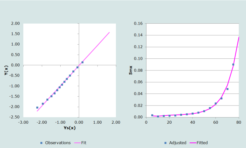
The coefficients α and β are determined as the intercept and slope, respectively, of the straight line fitted to the logit transformations in columns 4 and 6 of Table 4 over the range of ages chosen by the user (45 and 75 in this example), namely 0.0211 and 0.9672 respectively.
These coefficients are then applied to the logit transformation of the conditional model life table to produce the fitted logits in column 7 of Table 4. Thus, for example, the fitted logit at age 20 is calculated as follows:
These values are then used to produce the fitted life table in column 8 of Table 4. For example, the value at age 20 is calculated as follows:
The conditional years of life lived, Tx, which appear in column 9 of Table 4 are then calculated from the fitted life table and these numbers are used to produce the smoothed mortality rates which appear in column 10 of Table 4. For example, for age 80:
Diagnostics, analysis and interpretation
Checks and validation
The example above was taken from Manual X (UN Population Division 1983) which produced an estimate of completeness of around 83 per cent from application of both this method and the Preston-Coale method. The difference between these estimates and the one produced in this application (93 per cent) appears to be due largely to the method used to fit the line combined with the points used to fit the line. The Method sheet in the BGB_El Salvador workbook uses orthogonal regression while Manual X applied ‘grouped means’ to points up to age 60, and ‘trimmed means’ – thus effectively removing the impact of the final data point. This difference suggests that a case could be made for dropping the last two points in the example on the grounds that the regression is unduly influenced by points at the extremes of the axes. However, as indicated above, the effect of doing this when using orthogonal regression to fit the line is not particularly significant.
Interpretation
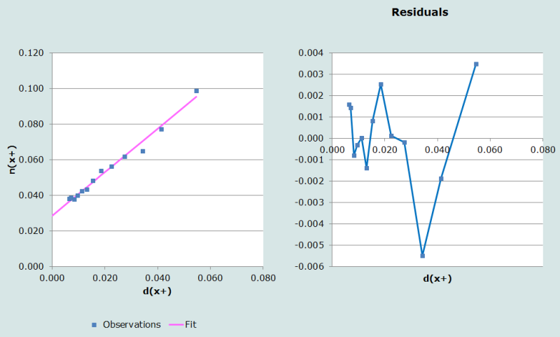
A problem that often arises with deciding on the ‘upper age’ for fitting the straight line is that estimates of completeness may vary quite considerably due to the exclusion of a single point. For example if one were to choose 70+ as the open interval the diagnostic plots would look as shown in Figure 4 and the estimate of completeness would be 82 per cent. The diagnostic plots, on their own, do not suggest that this fit is particularly worse than that using a 65+ open interval. In such cases one should calculate the estimate for several open intervals and use one which represents the estimate of completeness closest to the majority, or the median. Thus in this case the estimate of completeness for the open interval 60+ is 91 per cent, suggesting that the deaths are around 90 per cent complete. However, as pointed out above, as a general rule, it is not recommended in a population with significant digital preference to truncate at an age ending in zero.
Method-specific issues with interpretation
Source of reported deaths
Generally there are two sorts of problems with the deaths data: those that lead to under/over coverage that is constant by age, which is precisely what the method is intended to address, and those which lead to differential coverage by age, which can distort the estimates. Although the general approach remains essentially the same irrespective of the source of the death data, different sources of data are prone to different biases which might impact on the interpretation of the results. These differences are illustrated by way of particular examples, but, in general terms, you need to look out for the following biases in the death data.
1) Vital registration
If the proportionate split of the population between urban and rural (or appropriate proxies) areas differs significantly by age and the completeness of reporting of deaths in urban areas is significantly higher than it is in rural areas, then the assumption that completeness is independent of age is likely to be violated by a falling off of completeness with age at ages over 50, if a proportion of people move from urban to rural areas on retirement. If ignored, this violation is likely to lead to an underestimate of the average level of completeness.
2) Deaths reported by households in censuses/surveys
The data are subject to three potential problems:
- If a significant proportion of households dissolve on the death of a key person (e.g. the sole breadwinner), then the deaths of such people go unreported, leading to a violation of the assumption that completeness is invariant with age. If a significant proportion of deaths in some age groups are of individuals who do not live in private households (for example, they live in homes for the elderly), the breach of the assumption could be even more severe. However, this is not an issue in most developing countries.
- In situations where young adults leave the home they grew up in to work in urban areas, it is possible that they are regarded as being members of more than one household (or of neither household) and their deaths could be reported more than once (or not at all), again leading to a violation of the assumption of constant reporting of deaths by age. In this case, one can limit the impact by ignoring the data below a specific age in determining completeness.
- Reference period error: Since there is often confusion about the exact period for which deaths are to be reported, in addition to uncertainty about exact dates of death, it is possible for there to be overall under- or over-reporting of deaths. Provided one can assume that this is independent of the age of the deceased, this distortion will be accounted for in the estimate of completeness and is not a problem for estimating mortality rates.
3) Deaths recorded in health facilities
Little is known about how well this source of data works. However, it can be expected that completeness would depend on the distribution of health services from which the data have been gathered, and in many developing countries such services are likely to be concentrated in urban areas. So again, if the proportion of the population living in urban rather than rural areas varies with age, then completeness cannot be assumed to be independent of age. It is also possible that certain causes will predominate in facilities and, if these causes are significant and age-related, this could lead to a further violation of the assumption of constant completeness by age.
In all such cases, the plotted points will lie progressively above the fitted line at the older ages leading to an underestimate of completeness. The estimate will be improved, although still biased downward slightly, by excluding the points at the highest ages from determining the fitted line.
Detailed description of method
Mathematical exposition
Although the Brass Growth Balance method is simply a special case of the Generalized Growth Balance method, with the growth rate of the population aged x+, r(x+) constant for all ages, it might be of assistance to understanding these methods to describe the specific case as well.
Brass’s Growth Balance method (Brass 1975) has its origins in work by Carrier (1958) who first proposed a way of estimating mortality from the age distribution of deaths. The method derives from the relationship found in the balancing equation for a population closed to migration. In such a population the number of people in the population at time t2 is the number at time t1, plus the births that have occurred between time t1 and t2, less the deaths that have occurred between times t1 and t2, i.e. , where B and D are the births and deaths, respectively, that occurred between times t1 and t2. This equation can be generalized to hold for any population aged x and older, provided we have an estimate of the number of people who turned x (i.e. joined the age interval through aging) between the times t1 and t2, , and the number of deaths aged x and older that occurred between times t1 and t2, . Thus
(Equation 1)
If we rewrite equation (1) as
and divide through by the person-years of exposure between times t1 and t2 we can express the balance equation in terms of rates, i.e.
where
and
and are often referred to as partial or segmental birth and death rates, respectively.
These relationships only hold if there is complete and accurate recording of birthdays and deaths by age between times t1 and t2, and counting of the population by age at times t1 and t2.
Now suppose that all data are accurate except that the deaths are incompletely reported. Suppose further that one can assume (at least above a certain age – typically confined to adult ages) that a fixed proportion, c, of deaths are reported independent of the age of the deceased. Then , where represents the number of reported deaths aged x and older, and Equation (2) becomes , where
.
If we further assume that the population is stable, growing at a constant rate of r a year, then this equation can be rearranged as follows: . Thus, if one fits a straight line to the points , the intercept provides an estimate of the growth rate, r, and the reciprocal of the slope, k, provides an estimate of the completeness of reporting of the deaths, c.
Mortality rates by age group, , are then estimated as
Implementation of the method
Assume that in practice one has data on the following: the number of reported deaths over a number of years, from times t1 to t2, in five-year age groups, , up to an open interval at age A, ; and the number of people in the population in the middle of this period, in the same age groups, up to . These data can then be used to apply the method by computing and , and approximating or and .
If, instead of the population in the middle of the period, one had the population at some other time, say t, then one can apply the method using that population instead. The only difference is that the estimate of completeness will be relative to the population at time t as if it was the population as at the midpoint of the period. In other words, assuming the population to be stable, and the completeness relative to this population is the mortality rates derived by dividing the reported number of deaths corrected for this level of completeness by will give the same rates as one would obtain if one had had estimates of the population by age group in the middle of the period.
Fitting of the straight line
There are two aspects to determining the straight line that best represents the relationship between the partial birth and death rates, namely, the choice of method and the choice of points used to determine the slope and intercept.
Fitting the straight line using unweighted least squares regression is not recommended since this method gives too much weight to the values at the older ages, which tend to be less reliable. Thus, it is recommended that one fit the line using a more robust method such as the ‘mean’ line (i.e. the line defined as that joining the two points represented by the mean of the vertical axis values and the mean of the horizontal axis values of the first half and the second half of the age range) or the ‘trimmed mean’ line (i.e. the same as the mean line except that the average of the points is a weighted average - weighting the less reliable points, usually at the extremes, less than the other points). These methods are explained in detail in Manual X (UN Population Division 1983: 144-145). An alternative is described in more detail in the UN Manual on Adult Mortality (UN Population Division 2002: 105-110). The alternative is similar to the ‘mean’ line, except that one splits the range of points into three equally-sized groups1, and determines the line that joins the medians of the independent and dependent variables in the lowest third and the highest third of points.
Bhat (2002) points out that each method has its drawbacks and suggests, since it does not matter whether the partial birth or partial death rates are treated as dependent variable, that orthogonal regression is the best method for dealing with age misstatement. This reflects both vertical and horizontal distance from the line (by minimizing the orthogonal residual sum of squares (ORSS = ). Using this method c, the completeness of the death reporting, is estimated as the ratio of the standard deviation of the partial death rates to the standard deviation of the partial birth rates. The intercept is the mean of the partial birth rates, minus the mean of the partial death rates divided by c. This is the approach used in the applications of the Brass Growth Balance method in the accompanying workbook.
Limitations
The major limitations of the method as described above and provided for in the spreadsheet are that it requires that the population be stable and closed to migration and it should not be applied when these conditions do not apply to any significant extent. By way of example of inappropriate usage, application of this method (data available in the GGB_South Africa_males workbook) to estimate completeness of reporting of deaths in South Africa between the 2001 census and a census replacement survey in 2007, estimating the population in the middle of the period as the average of the two survey populations, provides an estimate of completeness, using the same age range, of 85 per cent. Increasing the minimum age of range of the data used to fit the straight line to 35 increases the estimate to 88 per cent, still somewhat lower than the estimate of 91 per cent produced using the Generalized Growth Balance method.
This method is less vulnerable to age misreporting than the Preston and Coale method. In particular, for example, the common tendency to exaggerate the age reported at death (relative to that recorded at census) will manifest itself by the plotted points falling off to the right (i.e. below the fitted line) over the range of exaggerated ages and this can be allowed for when deciding which points to use to fit the line. The method is, however, more vulnerable to the effects of destabilization resulting from a rapid decline in mortality (Martin 1980), in which case it tends to underestimate the extent of completeness since the lighter mortality is “interpreted” by the model as increased under-reporting (i.e. steeper slope). However, simulation has shown (Rashad 1978) that the bias resulting from a slow steady improvement in mortality (as has been experienced by some developing countries in the absence of epidemics, famine and wars) is quite small.
As far as changes in fertility rates are concerned, provided these have occurred not more than 15 years ago these changes will have little impact on the performance of the method since they affect mainly the youngest age groups.
Migration is likely to affect the young adult population (mainly between 20 and 35) but to have much less effect on deaths, which largely occur in old age. Unaccounted-for immigration will tend to lower the slope and hence lead to an over-estimate of the extent of death registration and an underestimate of mortality rates. Unaccounted-for emigration will have the opposite effect. Some demographers advocate fitting the straight line to data down to age 5 to limit the effect of unaccounted-for migration, on the assumption that any differences in completeness of reporting of deaths at these younger ages from that of the older ages is unlikely to lead to any major distortions since mortality is very light between ages 5 and 14. However, it is doubtful that this adaptation removes much of the bias.
Alternatively one could confine the fit to points above age 35 to remove the bulk of the effect of migration. However, often the data at the older ages is more suspect making the estimate of completeness less reliable. Although using these adaptations probably produces better estimates than simply ignoring migration, there is, unfortunately, little research into the accuracy of the estimated completeness produced by these adaptations.
Technically, if one had reliable estimates of net migration by age, one could adapt the method by replacing the partial birth rate b(x+) by b(x+) – i(x+), where i(x+) is the net in-migration rate, in deriving the fitted line. However, in practice, in situations where one has to apply this method one rarely has sufficiently reliable estimates of net migration by age to warrant adapting the method.
Fluctuations in the completeness of death registration with age are likely to introduce curvature in the pattern of points. Consequently, one of the strengths of this method is that if the points for successive age boundaries fall on a reasonably straight line, then it is probably reasonable to assume that completeness is constant with respect to age. However, where some but not all the points lie on a straight line one way of deciding which points to discard is to calculate the segmental growth rate for each successive open interval and then use those points for which the values of are reasonably consistent.
Perhaps the most important limitation of the method is that the plot of partial birth rates against partial death rates is, with the exceptions mentioned above, diagnostically quite limited. In particular, simulations of a demographically stable population which then suffers an increase in mortality due to HIV/AIDS with a population prevalence of 11 per cent, produce a plot of points which to all intents and purposes fit a straight line but underestimate the level of completeness, even if one confines the fit to ages over 45. The lesson is that, if the points do not fall on a straight line, there are problems with the data; however, if the points do fall on straight line, you cannot be certain that the estimates of completeness and coverage are correct.
Extensions
If one had accurate data and a reliable, independent, estimate of r (and the population is stable) then one could reformulate Equation 2 to estimate c(x+), the completeness of each open-ended age group, as follows: . However, in practice it is rare to find a sufficiently stable population with sufficiently accurate age reporting to make such an exercise worthwhile.
Further reading and references
Since this method is a particular case of the more general Generalized Growth Balance method, readers are referred to that section for further reading.
Bhat M. 2002. “General Growth Balance method: A reformulation for populations open to migration”, Population Studies 56(1):23–34. doi: https://dx.doi.org/10.1080/00324720213798
Brass W. 1975. Methods for Estimating Fertility and Mortality from Limited and Defective Data. Chapel Hill NC: Carolina Population Centre.
Carrier NH. 1958. “A note on the estimation of mortality and other population characteristics, given death by age”, Population Studies 12:149–163. doi: https://dx.doi.org/10.2307/2172187
Martin LG. 1980. “A modification for use in destabilized populations of Brass’s Technique for estimating completeness of death registration”, Population Studies 34:381–395. doi: https://dx.doi.org/10.2307/2175194
Rashad HM. 1978. “The Estimation of Adult Mortality from Defective Registration Data.” Unpublished PhD thesis, London: University of London.
UN Population Division. 1983. Manual X: Indirect Techniques for Demographic Estimation. New York: United Nations, Department of Economic and Social Affairs, ST/ESA/SER.A/81. https://www.un.org/development/desa/pd/sites/www.un.org.development.desa.pd/files/files/documents/2020/Jan/un_1983_manual_x_-_indirect_techniques_for_demographic_estimation.pdf
UN Population Division. 2002. Methods for Estimating Adult Mortality. New York: United Nations, Department of Economic and Social Affairs, ESA/P/WP.175. https://www.un.org/development/desa/pd/sites/www.un.org.development.desa.pd/files/files/documents/2020/Jan/un_2002_methodsestimatingadultmort.pdf
- Printer-friendly version
- Log in to post comments