The multi-exponential model migration schedule
Description of method in brief
This section describes how to fit a multi-exponential model migration schedule to observed migration data.
Over the last thirty years, these schedules, devised by Rogers and Castro (1981), have been remarkably successful in representing typical age patterns of migration. Essentially the same age patterns of migration have been observed whether national and interregional migrations are considered simultaneously, or migration from a specific region is considered in isolation. The multi-exponential function was designed to reflect the dependency between migration and age, and captures the relationship through an additive sequence of exponential curves, based on 7, 9, 11 or 13 parameters, depending on the complexity of the migration patterns and the ability and robustness of the data to sustain increased parameterization.
When fitted to a schedule of single-year-of-age migration rates, the Rogers-Castro model provides a best-fit, graduated expression of the migration schedule that finds application in smoothing an observed series of migration rates, and which can be used directly to enhance understanding of migration dynamics. The results can also find application in a number of alternative uses, for example, in setting migration schedules to be used in multi-regional population projections. Ideally, the analyst will have estimates of migration by single year and single ages to which the Rogers-Castro model can be fitted. However, if – as is often the case in developing countries where the quality of the underlying data may not permit such finely grained calculations – the data are only available in five-year age groups, then single-year age rates need to be interpolated from the data using one of the methods described in this chapter before attempting to fit a Rogers-Castro model.
Data requirements and assumptions
Tabulations of data required
- Migration propensities or migration rates by single ages from age 0 to an age above 65 (or if not in single ages, then by five-year age groups)
Ideally the data should be in the form of rates by single ages. Where they are in five-year age groups then single year observations must be interpolated from these five-year estimates before attempting to fit a multi-exponential curve. The choice of the upper age is somewhat arbitrary, but the upper bound of the data used in fitting a model schedule should – at the minimum – be greater than the modal age of retirement.
Important assumptions
Latest census counts the population by sub-national region and place of birth accurately and identifies who have moved from one region to another since a prior date (e.g. previous census).
Preparatory work and preliminary investigations
Before applying this method, you should investigate the quality of the data in at least the following dimensions:
- age structure of the population (by sub-national region as appropriate); and
- relative completeness of the census counts (by sub-national region as appropriate).
Caveats and warnings
Caution should be exercised in applying the method to net migration data, as the multi-exponential distribution of migration rates by age models gross migration flows (i.e. in- or out-migration) but not necessarily net migration, unless the flow in one direction significantly dominates the flow in the other at all ages.
Overview of the multi-exponential model migration schedule
The multi-exponential function was designed by Rogers and Castro (1981) to reflect the dependency between migration and age. High levels usually found in the first year of life. It drops to a low point during the early teenage years. Then it increases sharply to its highest point during the young adult years. After that, it declines, except for a possible increase and subsequent decrease during the ages of retirement. In some circumstances there may be an upward slope at the oldest ages (Rogers and Castro 1981; Rogers and Watkins 1987).
Over the last thirty years, the schedule (also known as the Rogers-Castro model migration schedule) has proven to be remarkably successful in representing age patterns of migration (Little and Rogers 2007; Raymer and Rogers 2008; Rogers and Castro 1981, 1986; Rogers and Little 1994; Rogers, Little and Raymer 2010; Rogers and Raymer 1999; Rogers and Watkins 1987). These same age patterns of migration have been documented for regions of different sizes and for ethnic and gender sub-populations (Rogers and Castro 1981). They appear whether national interregional migrations are considered simultaneously, or migration from a specific region is considered separately. Directional migration (i.e. from region i to region j) exhibit the same patterns as well. For example, the Rogers-Castro model migration schedule has been fitted successfully to migration flows between local authorities in England (Bates and Bracken 1982, 1987), Canada’s metropolitan and non‑metropolitan areas (Liaw and Nagnur 1985), and the regions of Japan, Korea, and Thailand (Kawabe 1990), and South Africa’s and Poland’s national patterns (Hofmeyr 1988; Potrykowska 1988).
When fitted to a schedule of single-year-of-age migration rates, the Rogers-Castro model provides a best-fit, graduated expression of the migration schedule that can be summarized by 7, 9, 11 or 13 parameters depending on the complexity of the schedule and strength of the data. In addition, the erratic fluctuations, often associated with unreliability in observed age-specific rates, are smoothed.
Rogers-Castro model migration schedules have been used in population projections in Canada (George 1994), and they have been imposed on time periods, regions, and subpopulations (Rogers, Little and Raymer 2010) when migration data were inadequate or unavailable.
The full model schedule has 13 parameters, which is the complete and most complex multi-exponential form of the model. If M(x) is defined as the migration rate for a single year of age x, the full model is defined as
It comprises five additive components. The first component, , is a single negative exponential curve representing the migration pattern of the pre-labour force ages. The second component, , is a left-skewed unimodal curve describing the age pattern of migration of people of working age. The third component, , is an almost bell-shaped curve representing the age pattern of migration post-retirement, where migration increases sharply following retirement before falling off again. Associated with this component, the fourth component is a single positive exponential curve of the post-retirement ages, , reflecting the (sometimes) observed generalised increase in migration post-retirement. This can be seen, for example, in the migration of the elderly in the US from the North-East to the “sunbelt” states in the South East and South West. The final component is a constant term, c, that represents ‘background’ migration.
Four families of multi-exponential schedules have been identified in past studies (Rogers, Little and Raymer 2010), and only one, exhibiting both a retirement peak and a post-retirement upslope, requires all 13 parameters and all five components. This family is documented in studies of elderly migration (Rogers and Watkins 1987), and is demonstrated in the bottom right panel of Figure 1.
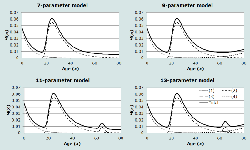
Source: Based on Raymer and Rogers (2008)
Note: The legend indexes, in order, (1) the pre-labour force migration schedule; (2) the working age migration schedule; (3) the post-retirement migratory increase and decrease; and (4) the generalised increase in post-retirement migration.
The other families are reduced forms of the full model, which means that at least one component is omitted. For example, the most common schedule identified by Rogers, Little and Raymer (2010) requires seven parameters and consists of the first two components and the constant term. This is also called the standard schedule, and its shape is set out in the top left panel of Figure 1.
A number of schedules have exhibited a standard profile plus a retirement peak (Rogers A and LJ Castro. 1981, 1986), resulting in the 11-parameter model, including components 1, 2, 3 and 5, shown in the bottom left panel of Figure 1. In populations with significant migrant labour, particularly in the developing world, it is possible that the third component is a trough rather than a peak, as migrants return home to retire.
The 9-parameter model is used when the standard pattern is visible for the labour and pre-labour force ages, and there is an upslope to represent migration in the post-retirement years as displayed in the top right panel of Figure 1. This was found in several regions of the Netherlands in 1974 by Rogers and Castro (1981).
As should be evident from the discussion above, all parameters are interpretable and can be used to characterize the model schedule.
In their original 11-parameter specification of the multi-exponential migration model, Rogers and Castro (1981) illustrated the model using data on male out-migration rates from Stockholm in 1974. Figure 2 shows the original data (the jagged lines) and the smoothed 11-parameter schedule fitted to the original data.
Five of the 11 parameters (α1, α2, α3, λ2 and λ3) give rates of change for different pieces of the model schedule while the level parameters (a1, a2, a3 and c) correspond to the heights of the model schedule. a1 gives the peak in the first year of life, a2 is the peak of labour force migration, a3 is the peak of retirement migration, and c gives the background migration rate. μ2 and μ3 give the ages at the labour force peak and at the retirement peak, respectively.
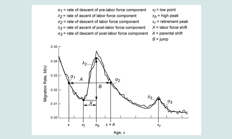
Some measures can be used to describe either the observed or the model migration schedule. For example, xl is the pre-labour force age when migration is at its low point. xh is the age when labour force migration peaks, and xr is the age of peak retirement migration. The difference between xl and xh is called the ‘labour force shift’, X, and the increase in migration rate between xl and xh is called the ‘jump’, B. A, the ‘parental shift’, is used to describe the average age difference between parent migration and the corresponding migration of children. The gross ‘migraproduction’ rate (GMR) is the sum of all rates over all ages (i.e. the area under the curve), and it is used to gauge the total level of migration out of a region or the total directional migration, i.e., from region i to region j (Rogers and Castro 1981).
Application of method
The method is applied in the following steps.
Step 1: Prepare a schedule of observed rates
The initial step in estimating a model schedule is to prepare the data. Decisions about which measure of migration to use depend upon the data sources available (registry, census, or survey) and the purpose of the research. For example, in a comparative study of migration patterns, any of the measures would be appropriate as long as they are constructed similarly across contexts. If, on the other hand, the model schedules are to be used in single-year population projections, the fitted schedule should represent single-age, single-year migration rates. However, where one does not have single-year single-age observations that produce progress relatively smoothly by age, then one must first convert the data one has into single-year single-age estimates. A number of commonly-encountered situations are described below.
a. Census data, annual migration rates, five-year migration interval
When the numbers of migrants who survived a five-year migration interval are available from census data which also give the year of most recent move, single-year, single-age migration rates can be derived through a conceptually simple, yet algebraically complex, back-projecting procedure outlined by Dorrington and Moultrie (2009). Their method compensates for the effect of mortality by applying the mortality regime of the general population to the migrants and for the effect of interregional migration by applying the annual rates of migration for the most recent year to estimate the population by region one year prior to the census and using that to estimate the migration rates two years before the census, and using that to estimate the population two years before the census, etc. It requires additional region-of-birth information for those aged 0-4 at time of census, as well as single-age, yearly estimates of regional populations. Schedules derived in this manner can then be fitted and smoothed with a Rogers-Castro model schedule, and used in single-year population projections.
b. Interpolating one-year from five-year age propensities
Regardless of the migration time interval, whether using census data or population register data, five-year age groupings generally give more reliable estimates of migration propensities than one-year age categories (Rogers, Little and Raymer 2010). In addition, counts of migrants in one-year age categories are typically only available from sample data, since national population bureaus tend to publish counts of interregional migrants in five-year age categories.
To apply the multi-exponential model when the initial migration proportions are in five-year age categories requires some method of converting the five-year rates to one-year rates. Cubic-spline interpolation (McNeil, Trussell and Turner 1977) is one such method that produces a smooth schedule for all integer values of ages. Rogers and Castro (1981) used data from Sweden, which was available in one-year and five-year age rates, to test the accuracy of the cubic-spline method, and found generally satisfactory results.
To arrive at smooth one-year age migration profiles, the initial migration proportions for the five-year age categories are assigned values close to the middle age within the five-year interval, i.e., ages 2, 7, 12, 15, … 72, 77 (or 2.5, 7.5, 12.5, …, etc., if estimating rates rather than probabilities). From this set of points, a continuous age profile of state outmigration propensities is generated with cubic-spline interpolation, which constructs third-order polynomials that pass through the set of pre-defined control points (called nodes). Commercial or freeware add-ins for Microsoft Excel, such as XlXtrFun, can also be used to implement cubic spline interpolation.
An alternative approach is to adapt Beers’ 6-parameter interpolation procedure (Beers 1945) to interpolate rates between the rates for the youngest and oldest age groups, which also extrapolates the rates to ages 0 and 1 (or 0.5 and 1.5 if working with rates). The extrapolation to the youngest ages is achieved by assuming that the difference between propensities for age 1 and 2 is the same as that between ages 2 and 3, and that between ages 0 and 1 is the same as that between ages 3 and 4.
Thus, to apply either approach one needs a set of migration rates in five-year age intervals from 0-4, to at least 65-69.
Step 2: Decide on the form of the multi-exponential model
Once the observed schedule is prepared, a decision must be made about the form of the multi-exponential model to be adopted. The overview of the multi-exponential model migration schedule presented above described the characteristics of the 7-, 9-, 11-, and 13-parameter models. This decision should be informed by a visual inspection of the schedule, keeping in mind that the model is assumed to represent the true form of the population migration schedule. Sometimes, even after plotting the schedule, it is not apparent how best to model the retirement years and the oldest ages. For example, it may appear that either a standard 7-parameter model or a 9-parameter model (increasing migration in the oldest ages) would be appropriate. In this situation, the decision in favour of the 9-parameter model could be based on a theoretical expectation for increasing migration in the later years. On the other hand, the 9-parameter model form might be rejected, based on the goodness-of-fit measures, as being insufficiently parsimonious if it produces no better fit than the 7-parameter model. In deciding which form of the model to use, it is recommended that the goodness-of-fit of the simpler model be compared with the more complex model, (e.g. comparing the fit of a 7-parameter model versus that of an 11-parameter model). As a general rule, and always bearing in mind the likely robustness of the underlying data, substantial improvement in fit is required to justify a more complex specification.
For most developing countries, particularly where ‘retirement’ isn’t concentrated between the ages of 60 and 65 and there is age exaggeration at the older ages, the data are probably not strong enough to fit anything more than the 7-parameter version of the model.
Step 3: Fit the model using Solver
Given the number of parameters (between 7 and 13) in the multi-exponential model migration schedule, determining a best fit ab initio using trial-and-error is not recommended. Instead, analytical algorithms have to be employed. The one described below uses an algorithm that is provided in Microsoft Excel, Solver. Solver may not be routinely loaded by standard installations of Microsoft Excel. To enable its use, proceed by selecting “File → Options → Add-ins → Manage Excel Add-ins → Go …” and then ensuring that the “Solver Add-in” is ticked.
The specifications of the Solver function, and the conditions and constraints that should be adhered to, have been set up in the workbook associated with the methods presented in this chapter. To run the routine on a given worksheet, select “Data → Solver → Solve”.
The model is fitted in the associated workbook and is set up to allow the user to set the “objective” to be minimized to be either the sum of squared differences between the observed rates and the fitted rates, or the chi-squared statistic.
The default Solver is set up to fit using all parameters. If one wants to fit a curve using only some of the parameters then one must specify only these parameters in the “By Changing Variable Cells” window, and set the other parameters to appropriate constant values (which may, or may not, be zero depending on the requirements of the fitting procedure). An instance where such constrained optimisation may be required is mentioned below.
The sum of squared differences is calculated as follows:
where Oi represents the observed rate at age i, Fi represents the fitted value at age i and n the number of age groups.
The chi-squared statistic is calculated as follows:
The chi-squared statistic is more sensitive to misfitting to age ranges where rates are lower (resulting in a proportionately larger error) and thus is a better metric to assess goodness-of-fit when trying to fit the ‘retirement hump’ (the third component).
Choosing initial estimates for the fitting procedure
The choice of initial parameter values is the principal difficulty in non-linear parameter estimation. Ideally, given a set of starting values, the algorithm proceeds through an iterative process, producing a revised set of “optimum” values. However, the optimum may be merely a local optimum, and not the global optimum. A better guess of the initial parameter values may produce an improved goodness-of-fit and produce a different set of final values. A poorer choice of initial parameters may prevent convergence to even a local optimum.
Bearing this in mind, the most effective method of ensuring that the results from a fitting procedure are indeed globally “optimal” is to choose parameter values previously reported for a “similar” curve. To this end one might start with the values already in the workbook which were used to fit the curves in the examples below.
Convergence may be more difficult to achieve with the 11- and 13-parameter models. Where such heavily parameterised models are justified, one approach that can be adopted is to first fit a standard 7-parameter model to the data (thereby securing the fit at the peak of the migration schedule, and at ages up to mid-adulthood). Then, one could proceed by fixing those 7 parameters to their estimates that resulted from the initial step (i.e. treat those parameters as constant from there on), and then estimate the remaining parameters. Another effective procedure is to carry out a linear estimation method first, which does not rely on an iterative algorithm. That method was first described in Rogers and Castro (1981) and later included as one of the several alternatives set out in Rogers, Castro and Lea (2005).
Another challenge in finding the optimum solution lies in choosing an appropriate stopping criterion for the iterative algorithm. As the iteration process converges on a solution, the chi-square statistic, which measures the differences between the observed and the estimated values, decreases. An indication that an acceptable solution has been found is when the chi-square value decreases by only a negligible amount from one iteration to the next. The level of this small difference is called the “tolerance” and is set by the user. The temptation is to set it to be a very small value, i.e. very close to zero, so that a true minimum chi-square value is achieved. However, the risk in this approach is that such a low tolerance may not be achievable, even when a solution has been found. Press, Flannery, Teukolsky et al. (1986) suggest a tolerance equal to .001 is a reasonable setting. If the estimation software fails to converge, the convergence criteria could be made less stringent, i.e. increase the tolerance, or try new initial estimates.
One trial-and-error method of choosing initial estimates makes use of the graphs in the accompanying Excel workbook. By substituting your schedule of observed data in one of the sheets, initial “guesses” of each parameter can be chosen and placed in the cells where the final estimates of each parameter are located. Then, by visual examination of the fit, and identification of the parameter values that are most out of line, try new initial values for those parameters and then re-evaluate the fit visually. Continue this way until the fitted schedule is reasonably close to the observed schedule. At this point, you will know you have reasonably good initial estimates and may proceed to the nonlinear least squares estimation procedure.
Step 4: Evaluate the model fit
We evaluate the model fit by calculating the mean absolute percent error (MAPE) statistic:
The MAPE is prone to overstate inaccuracy, particularly when the observed schedule has many values that are very close to zero (Morrison, Bryan and Swanson 2004).
In addition to MAPE, we also calculate R2, the square of the correlation between the Oi and the Fi values. A heuristic that is often employed is that a reasonable fit is achieved with a MAPE of 15 per cent or less together with an R2 well above 90 per cent.
In addition, since the method assumes the estimated Rogers-Castro model schedule represents the true form of the migration schedule, the estimated model schedule should appear to represent the underlying pattern of the observed data.
Step 5: Interpret the results of the fit
If the goal is to describe the pattern of migration and a multi-exponential model has been successfully fitted to the data, any of the summary measures (e.g. GMR, X, B, and A) as well as the parameter estimates can be used to describe the schedule. The summary measures and the parameter interpretations are given in the Overview.
Worked examples
In the examples below, multi-exponential model migration schedules are applied to a variety of data, of varying quality and complexity and from a number of different sources. All worked examples are provided in the associated workbook on the Tools for Demographic Estimation website.
Because iterative methods are required to fit a model life table to data on conditional survivorship in adulthood, detailed worked examples are not provided in the text. The reader is directed to the description provided in the previous section on how to use Solver in Microsoft Excel to determine optimal fits. The workbook is set up to use Solver to derive the results presented.
Census data, one-year migration interval
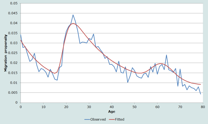
An example of a schedule based on one-year age migration propensities measured over a one-year migration interval from census data is shown in Figure 3. The data are derived from the 2005 American Community Survey (ACS), a national survey conducted annually by the U.S. Census Bureau. Even for California, a highly populated state, the one-year age propensities over a one-year interval are quite unstable. The MAPE is 17 per cent and the R2 is 0.92.
Caution must be exercised when using one-year age propensities over one-year migration intervals. For each single age, the numbers at risk of migrating, as well as the numbers of migrants, may be small, resulting in propensities that are erratic and unstable. A better option may be to derive five-year age propensities, which have proven to be more reliable than one-year age propensities (Rogers, Little and Raymer 2010). These can be interpolated to yield one-year age propensities using cubic splines or Beers’ formula as discussed in the section describing the application of the method.
Census data, five-year migration interval
Figure 4 shows an example using census data for the state of New Hampshire. The US Census Bureau’s 1 per cent Public Use Microdata Sample (PUMS) is a relatively small sample taken from the census and New Hampshire is one of the least populated states. The one-year age propensities appear to be quite unstable with dramatic fluctuations, while the model schedule provides a smooth estimate of the true schedule form. The MAPE is 52 per cent and the R2 is 0.68.
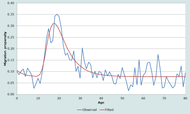
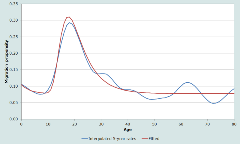
Figure 5 shows the cubic-spline interpolation method applied to the five-year age migration propensities for New Hampshire, derived from the 2000 Census 1 per cent public use microsample data. The schedule interpolated from the five-year age rates is much smoother and provides more reliable estimates than the observed one-year age rates displayed in Figure 4, and thus is a better set of estimates against which to compare the fitted multi-exponential curve. The MAPE was reduced from 52% for the one-year age propensities to 15 per cent for the rates interpolated from the five-year age proportions, and the R2 increased from 0.68 to 0.94.
There are several reasons why the levels of the New Hampshire schedule, in Figure 5, are substantially higher than the California schedule, Figure 4. The California example gives migration over a one-year migration interval and the New Hampshire schedule is over a five-year interval. In addition, New Hampshire is a much smaller areal region than California and the expectation is that the force of migration will be more powerful in a geographically smaller region.
Diagnostics, analysis and interpretation
Checks and validation
It is important to check visually if the age-specific migration rates have a ‘shape’ that is compatible with the Rogers-Castro models. If this is not the case then it is unlikely that these models will provide a satisfactory fit. Likewise, it is worthwhile checking whether there are any extreme values, particularly at older ages which might distort the choice of parameters or even the choice of the number of parameters to be fitted. If the observed estimates are particularly noisy, it would be better to group the data into five-year age intervals and then estimate a smoothed distribution using either the Beers 6-parameter interpolation provided or Spline curve fitting.
Considerations in applying the method
The formulation of the multi-exponential model was presented in the Overview and is not repeated here. In this section, we discuss in greater detail aspects that should be considered carefully before applying the method in practice.
Data preparation
The multi-exponential model is applied to schedules of one-year age migration rates beginning at age 0 and, typically, continuing to age 65 or higher to capture the full pattern of elderly migration. The schedules of age-specific migration might measure directional migration (i.e. from region i to region j) or total out-migration (i.e. from region i to all other regions), or all inter-regional migration with no specific origin or destination. Usually, migration data are obtained from national censuses (or, in developed countries, population registers). The multi-exponential model can be applied to a variety of measures of single-age migration propensities derived from either of these sources.
When obtained from national registration systems, the migration rate, for persons aged x at the beginning of the interval, is the ratio of the number of migrations during a given time interval divided by the average number of person-years exposed to the risk of moving. Persons can contribute more than one migration during the interval. These are occurrence-exposure rates, although migrations by non-survivors may not be included in the numerator (Rogers and Castro 1981).
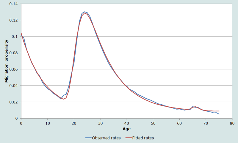
The observed migration schedule in Figure 2 was derived from Sweden’s national registry for male migration out of Stockholm over a one-year interval. In contrast, Figure 6 shows the observed and estimated model schedule for all male inter-communal migration in Sweden over a five-year interval. As expected, the levels are much higher in Figure 6 due to more migration activity when all regions are combined as compared to the Stockholm region alone. Similarly, more migrations are expected over a five-year interval than over a one-year interval. Rees (1977) found migration rates over a five-year interval tend to be less than five times (between 3 and 5 times) those over a one-year interval. The observed schedule is also smoother and more similar to the model schedule in Figure 6, indicating single-age migration rates are more reliable when based on a longer interval.
Censuses, on the other hand, count surviving migrants (not migrations). Migrants are persons who reported living in one region, at the beginning of the time interval, and resided in a different region at the time of the census. A person registering multiple migrations in a national register may be a non-migrant in the census if he returned to his initial location during the time interval. In general, counts of migrants from censuses understate the number of migrations, especially for longer time intervals when there are bound to be larger numbers of return movers and non-survivors. For these reasons, a migration schedule derived from population register data is not directly comparable to one based on census data (Rogers and Castro 1986).
Censuses typically record the location of a person’s current residence and ask where the person was living either one year ago or five years ago. Given this information and the person’s age at the time of census, the numbers of surviving migrants, and the numbers of survivors who were at risk of migrating are counted. The ratio of the number of surviving migrants to the number of survivors at risk for migrating is sometimes called a ‘conditional survivorship proportion’ because migrants and persons counted as being at risk for migrating must have survived the migration time interval to be counted by the census (Rogers, Little and Raymer 2010). Since these are not occurrence-exposure rates they will be called migration propensity here.
Census data, one-year migration interval
To derive single-age migration propensities when the census question asks where a person was living one year ago, all persons are “back-cast” to the region where they lived one year earlier when they were one year younger, which gives the number of persons at risk of migrating from that region. For example, a person aged 1 last birthday in a census conducted in 2010 would have been aged 0 last birthday in 2009. If the 2010 age values ranged from 1 to 85, they would range from 0 to 84 in 2009. (Note, only persons aged 1 and older would have reported place of residence 1 year ago.) Back-casting yields the number of people who survived to be counted by the census in 2010 and who were at risk for migrating from region i, in 2009. The number of migrants would be the count of persons who reported living in region i in 2009, but were counted as residing in a different region in 2010. For each 1-year age group, the ratio of the number of migrants to the number at risk for migrating gives the age-specific out-migration propensity for the 1-year interval. When the numerator contains directional migrants, i.e. from region i to region j, the ratio gives the age-specific propensity to migrate from region i to region j.
Caution must be exercised when using one-year age propensities over one-year migration intervals. For each single age, the numbers at risk of migrating, as well as the numbers of migrants, may be small, resulting in propensities that are erratic and unstable. A better option may be to derive five-year age propensities, which have proven to be more reliable than one-year age propensities (Rogers, Little and Raymer 2010). These can be interpolated to yield one-year age propensities.
Census data, five-year migration interval
When the census question asks where a person was living five years ago, it is possible to derive one-year age propensities for migrating over a five-year interval as long as single ages are reported. It is done by back-casting all persons to the region where they lived five years earlier when they were five years younger. Persons aged 5 last birthday in a census conducted in 2000, for example, would have been aged 0 last birthday in 1995. If the age values ranged from 5 to 85 in 2000, they would range from 0 to 80 in 1995. The number of migrants is simply the count of persons who reported living in region i in 1995, but were counted as residing in a different region in 2000. For each one-year age group, the ratio of the number of migrants to the number at risk for migrating gives the age-specific out-migration propensity over the five-year interval.
Census data, annual migration rates, five-year migration interval
When the numbers of migrants who survived a five-year migration interval are available from census data, single-year, single-age migration rates can be derived through a back-projecting procedure outlined by Dorrington and Moultrie (2009). Their method compensates for the effect of mortality by applying the mortality regime of the general population to the migrants and for the effect of onward migration by applying the annual rates of migration for the most recent year to estimate the population by region one year prior to the census and using that to estimate the migration rates two years before the census, and using that to estimate the population two years before the census, etc. It requires additional region-of-birth information for those aged 0-4 at time of census, as well as single-age, yearly estimates of regional populations. Schedules derived in this manner can then be fitted and smoothed with a Rogers-Castro model schedule, and used in single-year population projections.
Limitations
Unless one has accurate and well-behaved data the multi-exponential model will not produce a very close fit and thus can be over-parameterised – i.e. many different sets of parameters can produce virtually equally good fits to the observed values. In such a situation it might help to fix one or two parameter values and fit the rest, and parsimony with the number of parameters is recommended.
Extensions
Application of the multi-exponential model is not limited to schedules of migration rates or propensities. Several studies have established that age distributions of migrants (and migrations if using registration data) often have a multi-exponential form and can be accurately represented by a Rogers-Castro model schedule (Little and Rogers 2007; Rogers, Little and Raymer 2010).
The single-age numbers of migrants/migrations can be derived using any of the data sources and methods described above, because these are simply the numerators in the migration propensity and rate calculations. The observed data fitted by the model schedules are the single-age proportions of the total migrants/migrations. Note, if the numbers of migrants are reported in five-year age categories, some form of interpolation would be necessary. If cubic spline interpolation is used, the numbers associated with each node should be the migrants/migrations for each five-year age grouping divided by five.
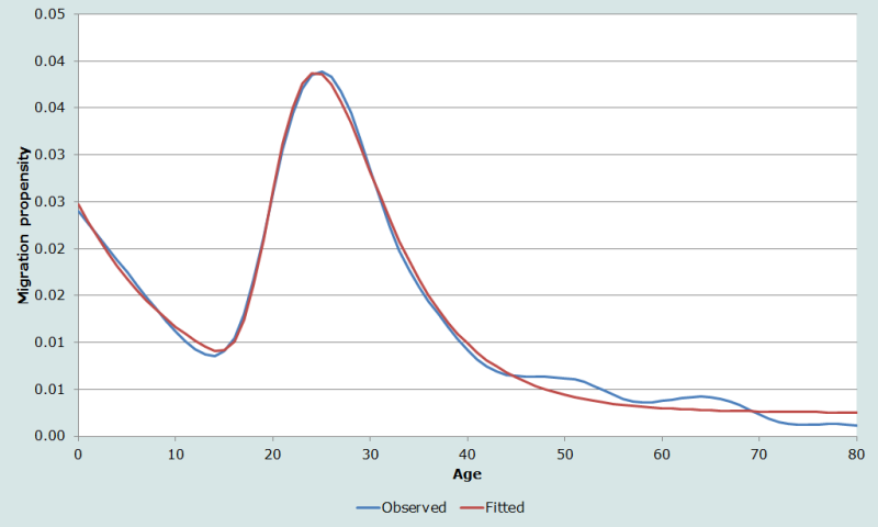
For example, the observed age composition of Swedish migrations as a proportion is illustrated in Figure 7. From this it appears to be very smooth and reliable except in the oldest ages. A 7-parameter model schedule fits pretty closely, with an R2 of 99 per cent and MAPE of 29 per cent. However, this is an example of the how the MAPE can exaggerate the model’s lack of fit, as it becomes inflated when there is a sequence of small observed deviations.
Two alternative software options for fitting to the Excel workbook for fitting the multi-exponential curve are 1) Data Master 2003, a free curve-fitting program, which applies the Levenberg–Marquardt algorithm; and 2) R (R Core Team, 2012) which is also free, but is a software environment for all-purpose statistical computing and graphics and as such requires a significant time investment before it can be used with confidence. The Appendix to this chapter on the Tools for Demographic Estimation website gives very basic commands for defining R-functions that produce estimates for the 7-parameter and the 11-parameter models using the Gauss-Newton algorithm.
References
Bates J and I Bracken. 1982. "Estimation of migration profiles in England and Wales", Environment and Planning A 14(7):889-900. doi: https://dx.doi.org/10.1068/a140889
Bates J and I Bracken. 1987. "Migration age profiles for local-authority areas in England, 1971-1981", Environment and Planning A 19(4):521-535. doi: https://dx.doi.org/10.1068/a190521
Beers H. 1945. "Six-term formulas for routine actuarial interpolation", The Record of the American Institute of Actuaries 33(2):245-260.
Dorrington R and TA Moultrie. 2009. "Making use of the consistency of patterns to estimate age-specific rates of interprovincial migration in South Africa," Paper presented at Annual Meeting of the Population Association of America. Detroit, Michigan, 29 April - 2 May 2009.
George MV. 1994. Population projections for Canada, provinces and territories, 1993-2016. Ottawa: Statistics Canada, Demography Division, Population Projections Section.
Hofmeyr BE. 1988. "Application of a mathematical model to South African migration data, 1975–1980", Southern African Journal of Demography 2(1):24–28. https://journals.co.za/toc/sajdem/2/1
Kawabe H. 1990. Migration rates by age group and migration patterns: Application of Rogers' migration schedule model to Japan, The Republic of Korea, and Thailand. Tokyo: Institute of Developing Economies.
Liaw K-L and DN Nagnur. 1985. "Characterization of metropolitan and nonmetropolitan outmigration schedules of the Canadian population system, 1971-1976", Canadian Studies in Population 12(1):81-102.
Little JS and A Rogers. 2007. "What can the age composition of a population tell us about the age composition of its out-migrants?", Population, Space and Place 13(1):23-19. doi: https://dx.doi.org/10.1002/psp.440
McNeil DR, TJ Trussell and JC Turner. 1977. "Spline interpolation of demographic data", Demography 14(2):245-252. doi: https://dx.doi.org/10.2307/2060581
Morrison PA, TM Bryan and DA Swanson. 2004. "Internal migration and short-distance mobility," in Siegel, JS and DA Swanson (eds). The Methods and Materials of Demography. San Diego: Elsevier pp. 493-521.
Potrykowska A. 1988. "Age patterns and model migration schedules in Poland", Geographia Polonica 54:63-80.
Press WH, BP Flannery, SA Teukolsky and WT Vetterling. 1986. Numerical Recipes: The Art of Scientific Computing. Cambridge: Cambridge University Press.
R Core Team. 2012. R: A language and environment for statistical computing. Vienna, Austria: R Foundation for Statistical Computing. https://https://www.R-project.org/
Raymer J and A Rogers. 2008. "Applying model migration schedules to represent age-specific migration flows," in Raymer, J and F Willekens (eds). International Migration in Europe: Data, Models and Estimates. Chichester: Wiley, pp. 175-192.
Rees PH. 1977. "The measurement of migration, from census data and other sources", Environment and Planning A 9(3):247-272. doi: https://dx.doi.org/10.1068/a090247
Rogers A and LJ Castro. 1981. Model Migration Schedules. Laxenburg, Austria: International Institute for Applied Systems Analysis. https://pure.iiasa.ac.at/id/eprint/1543/1/RR-81-030.pdf
Rogers A and LJ Castro. 1986. "Migration," in Rogers, A and F Willekens (eds). Migration and Settlement: A Multiregional Comparative Study. Dordrecht: D. Reidel, pp. 157-208.
Rogers A, LJ Castro and M Lea. 2005. "Model migration schedules: Three alternative linear parameter estimation methods", Mathematical Population Studies 12(1):17-38. doi: https://dx.doi.org/10.1080/08898480590902145
Rogers A and JS Little. 1994. "Parameterizing age patterns of demographic rates with the multiexponential model schedule", Mathematical Population Studies 4(3):175-195. doi: https://dx.doi.org/10.1080/08898489409525372
Rogers A, JS Little and J Raymer. 2010. The Indirect Estimation of Migration: Methods for Dealing with Irregular, Inadequate, and Missing Data. Dordrecht: Springer.
Rogers A and J Raymer. 1999. "Estimating the regional migration patterns of the foreign-born population in the United States: 1950-1990", Mathematical Population Studies 7(3):181-216. doi: https://dx.doi.org/10.1080/08898489909525457
Rogers A and J Watkins. 1987. "General versus elderly interstate migration and population redistribution in the United States", Research on Aging 9(4):483-529. doi: https://dx.doi.org/10.1177/0164027587094002
- Printer-friendly version
- Log in to post comments