Estimation of adult mortality from sibling histories

Available Data

Desired Result

Method

Description of method

This method calculates adult mortality directly from data supplied by adults on their siblings (that is brothers and sisters). It can only be applied when an inquiry has collected full sibling histories. Such histories ask each respondent for the name, sex, age, survival status and, if dead, age at and year of death of each of their siblings born to the same mother. Information on brothers is used to estimate the mortality of men and information on sisters to estimate the mortality of women. Many surveys only collect sibling histories from women, but sibling histories collected from male respondents can be analysed using exactly the same methods. As respondents and their siblings are about the same age, on average, sibling histories can be used to measure mortality over approximately the same range of ages as the ages of respondents that the histories are collected from.

Collecting sibling histories is a complex process that requires careful training and supervision of field staff to be executed correctly. It is not an appropriate methodology to use in a census. Many Demographic and Health Surveys (DHS) collect sibling histories (referred to by the DHS as the ‘Maternal Mortality Module’). While most of these surveys have only collected histories from women aged 15 to 49, as it is this group of women who complete a detailed individual interview, some DHS have collected sibling histories from men as well.

One advantage that sibling methods have over questions about household deaths is that only censuses or unusually large surveys can capture information on enough deaths in households in the year before the inquiry to yield mortality estimates that are sufficiently precise to be useful. Because respondents report on several siblings, on average, and one can calculate rates based on several years of exposure, estimates can be made from sibling history data in smaller inquiries. Nevertheless, all methods for the estimation of adult mortality require data on several thousand households. Another advantage of the method is that the estimation procedure makes few assumptions and, in particular, does not assume that the population being studied is closed to migration. However, the results from the method will not be representative for small states or sub-national areas in which a substantial proportion of the population are in-migrants or have emigrated.

Background

The initial methods developed for estimating mortality from information on the survival of siblings were indirect methods based on the idea that the average age of the siblings of respondents of any age is close to the age of the respondents. The proportion of a respondent’s siblings who are still alive is, therefore, a good estimator of life table survivorship to the age of the respondent (Hill and Trussell 1977; UN Population Division 1983). Unfortunately, field experience of this approach demonstrated that the quality of the data collected on siblings was often low because siblings who died before or shortly after the respondent’s own birth were often omitted by respondents, who may not know about them at all (Blacker and Brass 1983; Zaba 1986).

Interest in estimating mortality from data on siblings was revived by the development of the sisterhood method for measuring maternal mortality (Graham, Brass and Snow 1989). This requires data on how many sisters of the respondent survived to the age of 15, how many of them died thereafter, and whether sisters who died were pregnant at the time of death or had been pregnant during the 6 to 8 weeks before death. Limiting the consideration of siblings to only those who survived to age 15 years excludes siblings who died while still young and, therefore, may have been unknown to or forgotten by the respondent. The responses supplied to the first two of these questions by respondents in each five-year age group allow one to calculate the proportions still alive of sisters who survived to age 15. The indirect adult sibling method was subsequently developed so that the all-cause mortality of adult women could be estimated from these proportions still alive. Comparable data on respondents’ brothers can be used to estimate the mortality of men.

The method for estimating adult mortality by calculating life tables directly from full sibling histories collected from adult respondents was pioneered by the Demographic and Health Surveys programme based on this earlier research (Rutenberg and Sullivan 1991). It is more ambitious as to how much information it collects from the respondents and makes more demands on them and the field staff conducting the interviews. However, by replacing indirect estimation based on models of demographic relationships with the direct measurement of adult death rates, it reduces the number of assumptions involved in producing the estimates and, more importantly, allows one to separate deaths in the recent past from more distant ones, which may be reported on less accurately.

Data requirements and assumptions

Tabulations of data required

The calculation of mortality rates directly from sibling history data involves much the same steps and decisions as the more familiar process of calculating child mortality rates from birth history data – indeed, the history of a respondent’s full set of siblings, including the respondent, is the mother’s birth history. However, in comparison with mortality estimates made for children, estimates for adults have very large sampling errors. This reflects the facts that death rates are very much lower in adulthood than childhood and that, in a growing population, the number of siblings exposed to risk is small relative to the number of children reported on by mothers. In any household survey, therefore, far fewer sibling deaths than child deaths will be reported.

The calculation of cohort measures from sibling history data has little to recommend it either analytically or computationally, particularly given the ease with which modern survey analysis software can deal with the calculation of exposure times. Thus, this document focuses on the calculation of age-period death rates from sibling history data and on deriving other mortality indicators from them.

To calculate women’s mortality one needs to tabulate:

The number of deaths of respondents’ sisters by time period and five-year age group of the sisters at the time of their death
The number of sister-years of exposure by time period and five-year age group of the sister at the time of exposure.

To calculate men’s mortality one needs to tabulate:

The number of deaths of respondents’ brothers by time period and five-year age group of the brothers at the time of their death
The number of brother-years of exposure by time period and five-year age group of the brother at the time of exposure.

The calculations of exposure time should usually exclude the respondent himself or herself (and do so by definition if one is analysing sibling histories for the opposite sex). This requirement is explained in the discussion of the important assumptions made by the method.

Tables on respondents’ own-sex siblings (i.e. women’s sisters and men’s brothers) should be weighted only by any sample or design weights provided with the data. Tables on respondents’ opposite sex siblings (i.e. women’s brothers and men’s sisters) should be further weighted by the inverse of the number of surviving own-sex siblings of the individual respondent making the reports. This requirement is also explained in the discussion of the important assumptions made by the method.

The time period over which exposure is measured can be defined either in terms of calendar dates or relative to the date when the respondent was interviewed. The latter approach makes efficient use of the data as it ensures that the experience of respondents’ siblings during the incomplete years in which the interviews occur are included in the analysis. Calculating death rates for particular calendar years, however, has the advantage of yielding precisely time-referenced results that can be compared with those from other sources and is to be preferred. This approach usually entails discarding the data on the year in which the histories are collected but, if the majority of interviews took place late in that year, one might opt to include it in the most recent period.

The workbook is set up to calculate death rates for two successive periods prior to the collection of the data. Many DHS survey reports present rates for the seven-year period preceding their collection (that is, 0-6 completed years) and one way to use the spreadsheet would be to calculate rates for the three years prior to the inquiry and the four years prior to that. Alternately, death rates could be calculated for two four-year periods and for an eight-year period preceding the collection of the sibling histories. Experience suggests that the completeness of the reporting of dead siblings and accuracy with which their ages and dates of death are recalled often deteriorate rapidly for events occurring longer ago than that. Moreover, working with four-year periods rather than five-year ones minimizes errors that result from rounding of dates of death to five and ten years before the collection of the data.

The age groups of siblings for which the data are tabulated should broadly correspond to the ages of the respondents that the data were collected from. For example, in order to measure mortality between ages 15 and 60, one should ideally collect sibling histories from respondents aged 15 to 59. If data are only collected from adults, few of them have siblings that are still young children and, even if reports on children are not biased by failure to report some dead siblings, the estimates are likely to have large sampling errors and will not be representative of all young children. Thus, for DHS and other surveys that collect sibling histories from respondents aged 15 to 49, the preferred summary index of mortality is ₃₅q₁₅, the probability that someone aged 15 dies before their 50^th birthday.

Although the conditional probability of dying between ages 15 and 60 (₄₅q₁₅) is widely used by international agencies and other organizations as their preferred summary index of adult mortality, the number of deaths in the 55-59 year age group reported by respondents aged 15 to 49 will be small relative to those reported for younger age groups. Thus, rather than calculating ₄₅q₁₅ directly, it is better to do so by fitting a model life table to the estimates for ages 15 to 54 and extrapolating in this model to obtain mortality in the final five-year age group. This approach is implemented in the accompanying the workbook.

To eliminate ambiguities related to polygynous marriage and to remarriage, interviewers in most inquiries are instructed that ‘siblings’ means children born to the same mother. Whether or not this has been done, the reports should usually be accepted as they are. So long as respondents have the same group of relatives in mind when they are listing dead siblings as when they are listing those who are still alive, it is immaterial for the purpose of estimating mortality exactly who the parents of the siblings are.

If sibling histories have been collected from both men and women, their responses should usually be tabulated separately so that the two sets of data can be weighted appropriately and checked against each other.

Important assumptions

An inherent limitation of sibling-based methods for measuring adult mortality is that they underestimate mortality insofar as mortality clusters within sibships (i.e. sets of brothers and/or sisters born to the same mother). Clustering occurs whenever deaths are more concentrated in a small proportion of sibships than would be expected by chance and results from between sibship heterogeneity in individuals’ risk of dying (Zaba and David 1996). It causes downward bias in the mortality estimates simply because fewer members of a high mortality sibship than a low mortality sibship of the same size remain alive to answer questions about their siblings. It is impossible to correct fully for this because, at the extreme, sets of siblings whose members have all died are not reported on at all. Although one can assume something about them, there is no way of determining empirically from data collected retrospectively how many of these sibships existed or what their sizes were.

Estimates of the age pattern and trend in mortality will be biased if the extent to which mortality clusters within sibships varies with age. For example, if characteristics shared by sibs (e.g. genetic factors, early-life experiences, socio-economic status, life styles, and location) strongly influence the mortality of middle-aged adults, whereas mortality before age 40 has a large random component, estimates for older adults will underestimate mortality by more than those for younger adults, producing a spurious impression of mortality increase over time.

The issue of bias related to multiple reporting of siblings has received substantial attention in the literature. The problem exists in survey as well as census data because the more times an individual would be reported in a census, the more likely they are to be have a sibling who reports on them included in a probability sample.ⁱ Moreover, even in surveys, potential exists for multiple responses about the same individual. For example, if two daughters of the same mother are interviewed in the same household, there will be multiple reports about other members of the sibship. The standard approach to analysis used, for example, in DHS reports is based on the events and exposure time of reported siblings, leaving out the exposure time of the (surviving) respondent herself. Events and exposure time are weighted only by the respondent’s sample weight, not taking into account numbers of surviving potential respondents in the sibship.

Trussell and Rodriguez (1990) demonstrate mathematically that for groups of sibships with an identical underlying risk of dying, this standard approach yields unbiased estimates of mortality. In effect, the reduction in the number of deaths reported in the numerator that occurs because dead people cannot report on one another and the exclusion of the exposure time of the living respondents from the denominator offset each other precisely to give the correct mortality rates for the sibships as a group.

The issue of the biases that could result from differential mortality by sibship size is bound up with the issue of multiple-reporting bias. It has attracted a lot of research interest because, unlike other factors that affect risk within sibships classified by sex and age of the respondent, each respondent’s sibship size is known. If mortality does not vary with sibship size, the standard estimates are the same for every size of sibship, including one-person sibships that are excluded from the analysis because the respondent has nobody to report on, as well as for the population as a whole. Even if mortality varies by sibship size, the standard estimates remain unbiased for each sibship size, as pointed out by Masquelier (2013). To obtain mortality estimates for the population though, one must reweight the estimates for sibships of different sizes by the prevalence of sibships of that size in the population. When respondents are reporting on their own sex, one can achieve this by dividing the proportion of respondents from surviving sibships of each size by the estimated probability of surviving from the age at which siblings are counted as entering exposure to risk to the current age group of the respondents across all sibships of the same size. To do this for single-person sibships, their mortality has to be estimated by extrapolation from mortality in larger sibships.

Gakidou and King (2006) argue that, instead, sibships should include the exposure of the surviving respondent but should always be weighted in addition by the likelihood that they will be reported – that is, by the inverse of the number of potential respondents in the sibship. As in Masquelier’s approach, an adjustment also must be made for sibships that go unreported because no member remains alive. In a multi-survey analysis of DHS full sibling histories, Obermeyer, Rajaratnam, Park et al. (2010) estimate that the effect of not adjusting for the likelihood of reporting can bias overall mortality estimates downward by as much as 20 per cent.

Masquelier (2013), however, argues that Obermeyer and her co-authors reweighted their data files inappropriately and, as a result, exaggerated the size of any bias. He emphasizes that, if one is going to reweight, it is important only to adjust for multiple reporting by siblings who survived to the initial age from which mortality is being measured. In addition though, he questions whether the observed variation in mortality by sibship size is necessarily real. Instead, he argues, it may be an artefact of greater omission of dead siblings in the histories reported for large sibships. Masquelier therefore recommends using the standard approach, without attempting to reweight the data on each sibship. Then, either mortality should be estimated for each size of sibship and a reweighted estimate for the population obtained in the way described a few paragraphs previously or the estimates should not be reweighted at all. As making separate estimates for each size of sibship requires either a very large sample survey or fitting models to the data by regression methods in order to smooth them, the latter approach is adopted here.

When histories are being analysed on siblings of the opposite sex (for example, histories collected from women concerning their brothers), the issues are rather different. In this case, the respondent is not a member of the group that is exposed to the risk of dying. However, the standard calculation will still give biased results for the population as a whole if the mortality of siblings of one sex is associated with the number of siblings of the opposite sex that report on them. Thus, for reports on the opposite sex a clear case exists for weighting each report by the inverse of the respondent’s number of surviving siblings of their own sex as suggested by Gakidou and King (2006). Of course, questions about siblings of the opposite sex cannot generate any information on those sibships whose members have no living siblings of the respondent’s sex. Thus, adopting this approach is equivalent to assuming that the mortality of individuals in such sibships is the same as the mortality of the rest of the population. In surveys that collect data from both sexes, each sex supplies this information for the other and one can further weight the deaths and exposure reported by respondents by the inverse of the probability that siblings in each age group get reported on at all.

Preparatory work and preliminary investigations

The initial step in the analysis of sibling history data should be to assess the extent of non-reporting and incomplete reporting in the data set, in particular how many respondents stated that they did not know whether a particular sibling remains alive or simply failed to answer the question. It is also important to assess the extent to which the siblings’ dates of birth and ages, and their ages at and dates of death, are missing or have been imputed. If a lot of respondents failed to respond to these questions, the data supplied by those respondents who did answer them may not be representative of the population as a whole. Moreover, a high level of non-response may indicate that either the field staff or the respondents were having difficulty with the questions and it can be illuminating to determine whether the problem is concentrated among a minority of field staff or certain type of respondent. Heaping of reported dates and ages on particular ages and years also indicates that reporting is not very accurate. If the quality of the age and date data seems particularly poor, one might obtain better results from analysing the data set using the indirect adult sibling method.

If both women and men have been asked the relevant questions, one useful check on the completeness of the data is to assess how many siblings of each sex are reported, on average, by respondents of the other sex and whether the reported sex ratio at birth changes markedly as either the age of the respondent or the time since the birth of the siblings increases. It is fairly common to find that one sex (usually men) reports fewer siblings, and in particular fewer dead siblings, than the other. In other surveys, men and women may report similar numbers of siblings of each sex (after adjusting for the fact that respondents do not report on themselves) but that different numbers of them remain alive. The first type of discrepancy might result from differential age misreporting, but the second cannot.

Any bias due to clustering of mortality within families results in underestimates. Moreover, it seems unlikely that respondents invent siblings or report that their living siblings have died. Thus, the analysis should probably focus on the data supplied by respondents of the sex that reports most siblings and most siblings that have died.

Caveats and warnings

The only sibling methods that can be recommended produce probabilities of surviving from age 15 to ages later in adulthood conditional on being alive at exact age 15. In theory, it is possible to collect and analyse data on the deaths of siblings as children. Unfortunately, such reports are often very incomplete, particularly for siblings who died before or soon after the birth of the respondent. Thus, most applications of the method only attempt to measure siblings’ mortality at age 15 or more. To produce a complete life table, one has to estimate survivorship from birth to age 15 using another source of data.
Even in a large survey, the number of siblings that die each year in each age group is small. In most applications of the method, deaths and exposure need to be aggregated over several years in order to estimate death rates that are precise enough to be useful. Thus, the method is unlikely to be useful for detecting abrupt changes or fluctuations in adult mortality.
As one works backward from the time of the survey, the number of siblings exposed to risk diminishes rapidly, particularly at older ages. Moreover, respondents tend to omit some dead siblings from their reports, particularly deaths that occurred quite a long time ago. Thus, the histories tend to underestimate mortality and this bias often gets worse for estimates that are more distant from the time of the survey. Thus, the direct sibling method should not be used to estimate death rates for more than 10 years before the data were collected. Often only the data on the last seven years are analysed.
Given that the likelihood that dead siblings are omitted from the reports rises as the time since their death increases, the purpose of calculating rates for two periods before the survey is largely diagnostic. It enables the analyst to check whether the data indicate an implausible rise in mortality. One should be cautious about inferring trends in adult mortality from the internal evidence provided by a single set of sibling histories.
The direct procedure for estimating adult mortality from information on siblings does not involve the assumption that the population is closed to migration. Nevertheless, it can be difficult to interpret sibling-based estimates of adult mortality for sub-national geographic units, such as urban and rural areas or districts, or for respondents with particular socio-economic characteristics. This is because, although siblings usually share the same ethnic identity, many of the respondents’ siblings will live in different places from the respondents themselves and their socio-economic characteristics may differ from those of the respondents. Estimates for sub-national populations are also likely to have very large sampling errors.

Application of method

The procedure for estimating death rates from sibling history data is identical no matter whether one is analysing data on brothers, sisters, or siblings of both sexes and irrespective of whether the respondents are men, women, or both the sexes. The workbook is set up to calculate death rates for both brothers and sisters for two periods of time preceding an inquiry and for the entire period covered by them combined. Separate worksheets are provided for the analysis of data provided by male and female respondents. The workbook can produce estimates for periods of any length and for data tabulated by 'years before survey' or for calendar-year periods corresponding broadly to them.

Two tables are required in order to calculate the death rates for siblings of each sex reported on by respondents of a particular sex, which amounts to potentially four pairs of tables. One table should contain counts of deaths of siblings by year and age and the other table should contain person-years of observation of siblings exposed to the risk of death by year and age. The data can be tabulated for the age groups and periods that are going to be used in the analysis. Alternatively, one could produce the tables for single years of age and time so that the counts can be can be aggregated over either dimension into any set of wider intervals that is subsequently found to be of interest.

Assuming that data set lacks exact dates of birth for some siblings and exact dates of death for some siblings that have died, the most satisfactory way of addressing this limitation of the data is to impute exact dates using random numbers to place respondents within the range of dates at which the event could have occurred (Stanton, Abderrahim and Hill 1997). Survey organisations such as MeasureDHS may have done this before distributing the data from surveys that they conducted.

For imputation and analysis of the data on particular siblings to be possible, one needs to know either their year of birth or their current age, if they are alive, together with a year of death, age at death or time in years since death, if they are dead. If both the date of birth and date of death are incomplete, one would generally randomly assign the person an exact date of birth before assigning them a consistent date of death. Care should be taken to record the seed for the random number generator used for this, so that the imputed dates can be reproduced exactly if the need arises to recreate the data files being used to estimate mortality from the original data.

The details of the procedure that should be used to impute exact dates depends on precisely what questions were asked in the sibling histories about ages and times of death. A few examples will suffice to illustrate the principles involved in the calculations. If the respondent was interviewed on 23/11/2011 and reported that one of their siblings was 33 years old, that person’s date of birth must fall on or between 24/11/1977 and 23/11/1978. If a sibling is reported to have been born in October 1972 and to have died at age 17, one would first randomly assign them an exact date of birth, perhaps 14/10/1972, and then assign them an exact date of death on or between 14/10/1989 and 13/10/1990. If the respondent also reported a year of death for the sibling, the range of dates within which one randomly chooses a date of death should be restricted to the correct year.

A little care is needed to ensure that no siblings whose age at death equals the number of years since their birth are assigned a date of death later than the respondent’s date of interview. For example, if the respondent was interviewed on 28/2/2003 and reported that their sibling was born in 1980 and died at age 23, then that person must have been born in the first two months of 1980 and have died on or after that date in 2003, but before the end of February. The imputation procedure should also ensure that the imputed dates of birth occur in the correct temporal order of birth.

Once every sibling has been assigned an exact date of birth and, if they have died, of death, it is straightforward to identify the age groups in which deaths occurred and to divide the person’s life up between the age groups and periods (Stanton, Abderrahim and Hill 1997). Modern survey analysis software often contains commands that semi-automate this process.

Graphically, mortality is measured for the age group and period of time defined by the heavy lines in Figure 1. An individual’s life course by age and period is represented by the diagonal lines (as with a conventional Lexis diagram). The age group for which mortality is to be calculated is defined to have a lower bound of x_l, and an upper bound of x_h. The period of time for which mortality is to be calculated is defined as (t₂ - t₁), where t₂ is its end date and t₁ its start date. Thus, any person aged x at t₁ who does not die before t₂ will be aged x_t2 = x_t1 + (t₂- t₁) at time t₂. For statistics on adult mortality, both age and calendar time are almost always measured in years.

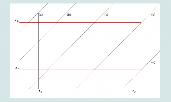
Figure 1 Lexis plane showing calculation of exposure to risk

Note that each sibling’s exposure in any year is almost always divided between two adjacent ages. Five possible scenarios are portrayed on Figure 1, labelled (a) through (e). Denoting the age at death of individuals dying in this age group and period as x_d, the contribution that each scenario makes to the person-years of exposure of the respondents’ siblings in this age group and period can be determined by the calculations shown in Table 1. Using these rules, one can calculate the exposure in the age group and period of each sibling reported on in the sibling histories. Summing exposure across all siblings gives total years of exposure to risk in the age group during the period, the denominator for the death rate. Summing the deaths occurring in the same age range and period provides the numerator for the rate.

Table 1 Algorithm for determining exposure to risk

Scenario	Description	Defining rule(s)	Exposure of survivors during the period	Exposure of decedents (if death occurs during the period)
(a)	Aged older than x_h at t₁	x_t1> x_h	0	0
(b)	Aged between x_l and x_h at t₁. Attains x_h in the period	x_l< x_t1< x_h x_t1+(t₂-t₁) > x_h	x_h-x_t1	x_d-x_t1
(c)	Attains x_l and x_h in the period	x_l > x_t1 x_t1+(t₂-t₁) > x_h	x_h-x_l	x_d-x_l
(d)	Attains x_l in the period. Period ends before x_h	x_l > x_t1 x_l < x_t1+(t₂-t₁) < x_h	x_t1+(t₂-t₁) > x_l	x_d-x_l
(e)	Does not attain x_l in the period	x_t1+(t₂-t₁) < x_l	0	0

Once the tables of deaths and exposure have been produced, various measures of mortality can be produced using standard life table calculations. These calculations are carried out for data on five-year age groups in the workbook. The age-specific death rate, ₅M_x, is calculated by dividing the deaths in a five-year age group in a specific year or period of years by the person-years spent exposed to the risk of dying in that age group during that period:

${}_{5}M_{x} = \frac{{}_{5}D_{x}}{{}_{5}N_{x}}$

The probability of dying in a five-year age group, ₅q_x, in the years concerned can be calculated from the corresponding death rate using the standard formula, which assumes that the deaths are evenly distributed across the age group:

${}_{5}q_{x} = \frac{5 \times {}_{5}M_{x}}{(1 + 2.5 \times {}_{5}M_{x})}$

The probability of surviving a five-year age group, ₅p_x, is 1 - ₅q_x.

From the series of estimates of ₅p_x, one can calculate the cumulative probability of dying between age 15 and age 50 for the period, ₃₅q₁₅, by multiplying together the intermediate five-year probabilities of surviving to obtain the probability of surviving from 15 to 50, ₃₅p₁₅, and subtracting this probability from 1 to obtain its complement:

${}_{35}q_{15} = 1 - {}_{5}p_{15} \times {}_{5}p_{20} \times {}_{5}p_{25} \dots \times {}_{5}p_{45}$

The 95 per cent confidence intervals of these summary measures of adult mortality provided in the Excel workbook are calculated using Greenwood’s formula. This formula assumes that the data are generated from a simple random sample and so will overstate the precision of indices based on data from cluster surveys.

The workbook produces plots of the logits of the conditional probabilities of surviving from age 15 to each higher age against the equivalent values of logit survivorship in a standard life table. Such plots are useful for evaluation of the quality of the estimates. Data errors usually show up as irregularities in the series or in the form of downward curvature of the series in the oldest age groups. The latter pattern is indicative of underestimation of mortality due to exaggeration of ages and ages at death.

Finally, the workbook fits a 2-parameter relational model life table to the series of _np₁₅ values by means of a simple linear regression across the entire age range 15 to 55 years. This smoothes out some of the errors in the series. Fitted values of ₃₅q₁₅ and₄₅q₁₅ are extracted from this life table. The workbook can fit the model life table and calculate these mortality indices using either a standard from the General family of United Nations model life tables (UN Population Division 1982) or one from any of the four families of Princeton model life tables (Coale, Demeny and Vaughan 1983). The standard life table should be chosen to have an age pattern of mortality within adulthood that resembles that of the population being studied. Another life table can be used as a standard if there is reason to believe that it resembles more closely the pattern of adult mortality in the population being studied. The most suitable life table may not be from the family of models that best captures the relationship between child and adult mortality. If nothing is known about the age pattern of mortality in adulthood, use of the United Nations General or Princeton West models is recommended.

Worked example

These calculations are illustrated in Table 2 using data collected from female respondents about their sisters in the 2001 Maternal Mortality Survey of Bangladesh (available on the DHS website). Note that this is an unusually large survey. The deaths and exposure of the respondents’ sisters in each five-year age group have been cumulated across the seven-year period preceding the survey. After the calculation of the death rates and estimates of life table survivorship, the latter have been smoothed by fitting a 2-parameter relational model life table using a Princeton South model life table as the standard.

Table 2 Direct calculation of age-specific death rates and the probabilities of dying between age 15 and ages 50 and 60, women, Bangladesh, 1994-2001

Age group x to x+4	Deaths of sisters	Person-years of exposure	Age-specific death rate ₅M_x	Five-year survivorship ₅p_x	Cumulative survivorship _x-10p₁₅		Logits _x-10Y₁₅	Smoothed logits _x-10Y₁₅
15-19	350.3	211840.6	0.00165	0.9918	0.9918		-2.3956	-2.4318
20-24	436.8	241208.5	0.00181	0.9910	0.9828		-2.0235	-2.0109
25-29	488.0	241111.4	0.00202	0.9899	0.9729		-1.7909	-1.7758
30-34	455.0	210963.3	0.00216	0.9893	0.9625		-1.6225	-1.5978
35-39	417.5	160378.1	0.00260	0.9871	0.9500		-1.4727	-1.4472
40-44	377.5	97268.6	0.00388	0.9808	0.9318		-1.3072	-1.3020
45-49	242.0	50456.1	0.00480	0.9763	0.9097		-1.1550	-1.1581
50-54	169.4	19621.2	0.00863	0.9577	0.8713		-0.9561	-1.0002
55-59	56.7	6276.6	0.00904	0.9558	0.8328		-0.8027	-0.8286
₃₅q₁₅ (95% CI)			0.090	(0.086 - 0.094)		(α =	-0.191)	0.090
₄₅q₁₅ (95% CI)			0.167	(0.155 - 0.179)		(β =	0.949)	0.160

Plots of the estimates against the standard are shown for the sisters, distinguishing between the periods 0 to 2 years and 3 to 6 years before the survey, in Figure 2. The equivalent plots for the respondents’ brothers are shown in Figure 3. For these particular data, the smoothed estimates of ₃₅q₁₅ and₄₅q₁₅ are almost identical to the estimates calculated directly from the data at 90 per 1000 and 167 per thousand respectively.

Diagnostics, analysis and interpretation

Checks and validation

If sibling histories have been collected from both men and women in a census or a large survey, analysing them separately for male and female respondents can be recommended in order to compare the consistency of their reports. The mortality of individuals of a particular sex, as reported by their brothers, should be the same as the mortality of the same individuals as reported by their sisters. If it is not, this may indicate significant bias in the estimates for one or both sexes. While consistency of reporting does not guarantee accuracy, statistically significant differences between the estimates obtained from male or female respondents do imply that at least one sex, and possibly both of them, are answering the questions inaccurately. This check on the results cannot be carried out on the data from the 2001 Bangladesh Maternal Mortality Survey as sibling histories were collected only from women in this study.

Interpretation

The results of the illustrative application of direct calculation of death rates from sibling histories using data from the 2001 Maternal Mortality Survey of Bangladesh are shown in Figures 2 and 3. They are encouraging. The plotted points are not at all erratic and do not curve away at older ages. There is some curvature in the series for men, particularly for the earlier period, but this spans the entire series of points from age 20 up to age 60, rather than affecting just the older ages. It probably indicates that the age pattern of mortality in this population differs from that in the standard life table.

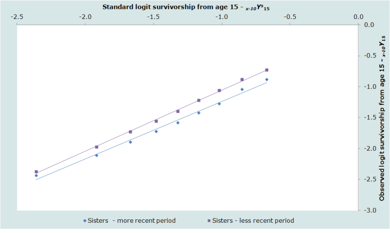
Figure 2 Logit survivorship from age 15 plotted against a Princeton South model life table, women, Bangladesh, 1994-2001

The estimates for the two periods are consistent with each other for both sexes, in each case suggesting that adult mortality declined substantially during the 1990s. Thus, the probability of dying between ages 15 and 50 of men is estimated to have dropped from the 104 per thousand to 76 per thousand between the period 3 to 6 years before the survey and 0 to 2 years before the survey. The probability of dying between ages 15 and 50 of women dropped from 107 per thousand to 73 per thousand between the same two periods.

Figure 3 Logit survivorship from age 15 plotted against a Princeton South model life table, men, Bangladesh, 1994-2001

Although the overall probability of dying between ages 15 and 50 in Bangladesh is very similar for men and women and has declined at a similar rate for both sexes, Figures 2 and 3 reveal that Bangladeshi men and women have very different age patterns of mortality within adulthood. Mortality rises much more steeply with age for the men than the women. The β parameter of the model life table fitted to the 1994 to 2001 data for women is 0.95 while, in the equivalent model life table for men, it is 1.14. Thus, if one examines the death rates for the five-year age groups, they show that women have higher mortality than men in Bangladesh at ages 15 to 40, but that men in their 40s and 50s have higher mortality than women.

The internal regularity of each of the four series of estimates from this survey in Bangladesh, the consistency of the estimates for the two periods before the survey, and the plausibility of the age pattern of mortality as assessed against external standards, all represent evidence that the method worked well in this survey. The most surprising feature of the results is the very large drop in adult mortality that they suggest occurred in Bangladesh in the second half of the 1990s.

Performance in populations with generalized HIV epidemics

The HIV epidemic poses two problems for methods of estimating mortality based on the survival of relatives (UN Population Division 1982). First, both the sexual and vertical routes of transmission produce significant selection biases in data collected in surveys on the survival of relatives. Second, the incidence of HIV infection is concentrated among young adults. Thus, populations with significant AIDS mortality have very different age patterns of mortality from both other populations and existing systems of model life tables.

A major advantage of sibling methods of measuring adult mortality over questions about other relatives is that they are free of selection biases arising from direct transmission of the virus. Some residual bias due to clustering of AIDS mortality within sibships will remain. All the children born to a woman after she becomes infected are at risk of infection by vertical transmission. Moreover, the risk of HIV infection tends to vary markedly between localities and siblings often live close to each other. The impact of this, however, will be relatively small compared with the biases that affect data that parents have supplied about their children or vice versa. Moreover, direct estimates of mortality from sibling histories have an advantage over the indirect adult sibling method in populations with substantial AIDS mortality in that they measure the age pattern of mortality directly – nothing has to be assumed about it.

Extensions and variants of the method

In order to extract the maximum useful information from sibling histories in the presence of both reporting and sampling errors, analysts have resorted to multi-country analyses of sibling-level data files using regression models to impose some discipline on the results (for example, Obermeyer, Rajaratnam, Park et al. 2010; Timæus and Jasseh 2004). For instance, Timæus and Jasseh incorporate a 2-parameter standard mortality schedule in their regression model of the log mortality rates in order to smooth the data. They allow the regression coefficient for the standard (which determines the age pattern of mortality) to vary between countries but not to change over time. Moreover, they assume that, while the speed of decline in mortality from causes other than AIDS varies between countries, it follows a log-linear trend in them all. Other analysts have constrained their estimates in different ways.