General assessment of age and sex data
Introduction
“In a perfect world, data would always be complete, accurate, current, pertinent, and unambiguous. In the real world, data are generally flawed on some or all of these dimensions” (Feeney 2003: 190). The task of evaluating and assessing data is an essential part of identifying the nature, direction, magnitude and likely significance of these flaws. While the primary point at which data evaluation and assessment takes place is immediately after the data have been processed, data evaluation and assessment are recursive activities – at each analytical stage, the user of demographic data should consider the results produced with a sceptical eye, alert to possible indications of error or bias introduced by the data into the results.
Here we set out the essential investigations that should be carried out as a matter of course before embarking on a process of demographic analysis. The basic principles for performing demographic evaluation and assessment have barely changed in the last half-century. Accordingly, aspects of the material presented in this section have been drawn from the United Nations’ Manual II: Methods of Appraisal of Quality of Basic Data for Population Estimates (UN Population Branch 1955), updated and modified as appropriate, as well as from another, more recent, guide to the evaluation of census data, the US Census Bureau’s guide, Evaluating Censuses of Population and Housing (U.S. Bureau of the Census 1985). The latter work provides a comprehensive and useful guide to the subject; in particular, Chapters 4 and 5 are strongly recommended to all analysts setting out on a process of data assessment and evaluation of demographic data.
The next section explains why it is necessary to evaluate demographic statistics. It also provides a high-level overview of the principles and practices involved.
The need for appraisal of demographic statistics
Population statistics, like all other demographic statistics, whether they are obtained by enumeration, registration, or other means, are subject to error. The errors may be large or small, depending on the obstacles to accurate recording which are present in the area concerned, the methods used in compiling the data, and the relative efficiency with which these methods are applied. The importance of the errors, given their magnitude, depends on the uses to which the data are put. Some applications are valid even if the statistics are subject to fairly large errors; other applications require more accurate data. When dealing with any given problem, it is important to know whether the data are accurate enough to provide an acceptably accurate answer.
For population estimates, evaluation of the census or registration statistics on which the estimates are based is doubly important. In the first place, an investigation of the accuracy of the base data is a prerequisite to any attempt at determining the reliability of the estimates. Errors of estimation result both from inaccuracies in the basic population statistics and from errors in the assumptions involved in deriving the estimates (for example, in the assumed population changes between the date of the latest statistics and the date to which the estimate applies). Both sources of error must be taken into account if the degree of confidence that may be placed in the estimate is to be known. Second, where an investigation into the accuracy of the base data has revealed errors, the direction and magnitude of which can be estimated, it is possible to make explicit or implicit compensating adjustments, as the estimates of population are prepared. It is often the case, too, that reasonably reliable demographic measures (for example, fertility rates) can be derived, even when the underlying data are unreliable on some dimensions.
The purpose here is to describe the basic methods for appraising the accuracy of those aspects of the census data most commonly used as a basis for current population estimates and future population projections. It is assumed that the results have been compiled from at least one census, and that the analyst is faced with the problem of determining the accuracy of the census and other population data, but is not in a position to re-enumerate the whole population or repeat any major part of the census undertaking.
It is not possible to consider in every detail all the possible information which, in a given country, can be utilized for an appraisal of its demographic data. For example, survey data may provide estimates of demographic parameters that would be valuable in evaluating the quality of data from a census. Hence, the examples presented here should be regarded as illustrations of methods and the results should not be taken as definitive evaluations of the quality of the particular data employed.
The results of the tests described in this manual are of various kinds. Sometimes, a test will reveal only that statistics are either "probably reasonably accurate" or "suspect"; if they are "suspect" further intensive investigation is required before a definite judgment can be made. Other tests will not only indicate that errors are present, but also lead to an estimate of the direction and probable extent of the error. In the latter case, it is desirable to adjust or correct the faulty statistics and to revise the estimates based on them. The description of procedures to be used in the revision of estimates, however, is outside the scope of this manual.
The distinction that is often drawn in demographic texts between coverage errors (introduced through differential enumeration across regions, ethnic groups, ages etc. leading to the data set being unrepresentative of the statistical whole it is meant to represent) and content errors (introduced through respondent or enumerator error, or misreporting) is not particularly helpful in determining strategies for data assessment. In many instances flaws in the data may not be attributable solely to one or the other kind of error. However, in seeking to explain and understand the errors identified, it is useful to consider where in the census process the error may have been introduced. Doing so assists in the determination of appropriate remedial courses of action to correct the data if possible. The description of such remedies is again outside the scope of this manual.
Background documentation that should be sought
The process of conducting a census is arduous and complicated – it has been claimed, for example, that the decennial census conducted in the United States is the largest and most complex peacetime undertaking of the Federal Government (National Research Council 2004). The same is probably true in any other country conducting a census. To assist with the task, recommended standards and procedures have been drafted by the United Nations Statistics Division. Many of the relevant manuals are available online: the two of greatest interest to demographers analysing and evaluating the quality of census data are the Principles and Recommendations for Population and Housing Censuses, Revision 2 (UN Statistics Division 2008) and the Handbook on Population and Housing Census Editing, Revision 2 (UN Statistics Division 2020). The former offers guidance on the logistics of conducting a census, from planning all the way through to dissemination; the latter deals with the post-enumeration handling of the data in preparation for release.
The nature and quality of the demographic data available varies greatly between countries. Population censuses are undertaken with varying frequency and accuracy, and vital registration data contain widely divergent levels of detail, and vary hugely in quality between and within countries. Migration across national boundaries may be relatively important or not. Consequently, different methods have to be employed in different situations for the appraisal of the accuracy of statistics, and it is therefore not possible to consider all the detailed tests to which every conceivable kind of data on the subjects covered here can be submitted. The methods presented here may, therefore, not always be directly applicable to a specific problem; modifications must be identified to suit particular requirements.
Where possible the analyst should seek to obtain as much relevant information as possible from the agency responsible for conducting the census or survey regarding operational practices and difficulties experienced, as well as the policies and practices adopted for cleaning and editing the data prior to release. Where a post-enumeration study has been conducted, information on this should also be obtained.
In addition to data sources that may not be in the public domain, the quality of the insights gained into the nature of the data will depend on the ability of the analyst to bring to bear on the data as much potentially relevant material, not only demographic, but also social, economic, historical and political information as possible. As a simple example (more on which below), the dramatic decline in adult survival probabilities in the late 1990s indicated by the data from the 1992 and 2002 Zimbabwean Censuses can be explained in large measure by the effects of HIV/AIDS on adult mortality at that time.
Types of testing procedures
Whether one is dealing with census data, vital statistics, or records of migration, the same basic types of testing procedures are applicable. This similarity arises from the fact that demographic phenomena are interrelated both among themselves and with other social and economic phenomena. Some of these relationships are direct and necessary. For example, the increase in population during a given interval is precisely determined by the numbers of births, deaths, and net migratory movements occurring in that interval. Other relationships are less precise and less definite. For example, in some countries, an economic depression is likely to result in a declining, and prosperity in a rising, birth rate, but the exact amount by which the birth rate will change cannot be inferred even from detailed knowledge of the economic situation.
The basic types of possible testing procedures can be summarized as follows:
- consistency checks, based on one or more censuses;
- comparison of observed data with a theoretically expected configuration, for example the use of balancing equations and population projection models;
- comparison of data observed in one country with those observed elsewhere;
- comparison with similar data obtained for non-demographic purposes; and
- direct checks (re-enumeration of samples of the population etc.).
The first type of checking procedure examines the consistency of the data, either internally (for example, does the distribution of the population by age and/or sex conform to expectations), or externally by means of comparison with earlier data from the same country. Demographic transition theory leads us to expect that – typically – birth rates and death rates (and hence population growth rates) will decline in a coherent, orderly fashion, without major discontinuities. (The exception is the likelihood that, at the very start of the transition, birth rates may rise). In the absence of clearly identifiable exogenous factors (e.g. war, famine or epidemics), deviations and departures from this orderliness therefore held strongly suggest problems in the data.
Comparisons of the second type have changed significantly over the years. Historically, the most common tests of this type were to compare the data against those implied by a stable-population equivalent of the country in question. With the onset of fertility decline in almost every country in the world, the assumptions necessary for comparisons of this type to produce meaningful results have become increasingly invalid. Contemporary comparisons of this sort now more frequently seek to compare male and female mortality rates and sex ratios by age with those that would be anticipated in contexts similar to those of the source of the data being investigated. In addition, comparison with the results of model outputs (for example, the United Nations’ World Population Prospects or the US Census Bureau’s projections) can be used to highlight possible inconsistencies in the data.
"Balancing equations" can also be applied to test the consistency of the increase in population shown by two enumerations at different dates, using the increase shown by statistics of the various elements of population change—births, deaths, and migration—during the interval. If all the data were accurate, the two measures of increase (or decrease) should be balanced. Aside from population totals, the test can also be applied to sex and age groups and other categories of population that are identifiable in the statistics. Furthermore, by rearranging and re-defining the components of this equation, separate appraisals can be made regarding the accuracy of birth, death and migration statistics.
The third type of test relies on prior knowledge of a country that is expected to be demographically similar to the country of interest. This may, for example, be a neighbouring country. However, great care must be taken if this approach is to be adopted to ensure that the similarities between the two countries are sufficiently great (not only demographically, but also socially, economically, culturally etc.) to permit the extrapolation of data from one demographic setting to another.
The second and third types of check are similar. The demographic changes observed in another country where conditions are presumed to be similar can sometimes be substituted for a theoretically expected configuration. In both cases, the comparisons will differ, whether by a large or a small amount. The essence of the test then rests on the answer to the question: Can the difference between the observed and expected values be explained by historical events or current conditions in the country, the data of which are being tested? If not, then it must be concluded that the observed data are "suspect". Further investigation may yield an explanation of the difference, or it may furnish clear indications that the "suspect" data are indeed in error. Very often this kind of method is applied as a preliminary step, to suggest along what lines further testing should be undertaken.
The fourth type of test relies on the availability of administrative or other social statistics that may shed light on the demography of the country of interest. Estimates of the sizes of different components of a national population might be obtained from voters' registers, school enrolment statistics, select populations such as Demographic Surveillance Sites (DSSs), etc. If such estimates differ from the population census data, the question arises whether there is a satisfactory explanation for the difference. Given the dependency on the specifics of the local data available, and the nature of the comparisons that might be drawn, tests of this type are not discussed further here. However, care must be taken not to assume these alternative sources are necessarily better than the census being checked.
Finally, direct checks involve a field investigation, such as a post-enumeration survey. The advantage of a direct check consists in the fact that the individual persons enumerated, or the individual events registered, can be identified, so that not only the consistency of totals, but the specific errors of omission or double-counting come to light. Direct checks in the form of a post-enumeration survey also allow for the correction of the enumerated population for an estimated undercount.
The first four types of testing procedure give an indication only of relative accuracy as both sets of data may be subject to error. If several testing procedures are applied, or if there is a strong presumption that one set of data used in the comparison is highly accurate, the evidence so secured provides a strong indication that the data being tested are inaccurate. In many other instances, the comparison may only reveal that at least one, if not both, sets of data are in error.
The investigations described below concentrate on the first and second types of test. (Direct checks are discussed briefly elsewhere, in the section on post-estimation consistency checks). Wherever possible, specific examples are included. The data for these examples have been drawn from the census data held at IPUMS (Minnesota Population Center 2015). However, only a fraction of the data and knowledge available in each country was used in working out these examples. Many more relevant data, some of them not published anywhere, exist in these countries.
A final observation before proceeding to the description of the various tests described here: most (although not all) of the tests can be applied at smaller geographical subdivisions, with the caveat that migration plays an increasingly significant role in determining the size and shape of populations at smaller levels of disaggregation. Here, too, we expect to find "orderly" patterns of population change, both within the same subdivision in successive intercensal periods, and among different subdivisions in any period. Any dissimilarities should be explicable in terms of known conditions. As a practical matter it is well known that there may be considerable diversity in the rates of population change among the various parts of any nation. Accordingly, the problem becomes one of trying to distinguish between changes which are explainable in terms other than errors in the statistics and those which are not. It should be noted that although these procedures may reveal the presence of errors and in some cases indicate their order of magnitude, they do not provide a basis for exact estimates of the size of the errors.
Preliminary checks
Before trying to assess the quality of the data the analyst should:
- Review the census enumeration procedures and information on the quality of performance, including ascertaining whether a post-enumeration survey was done, and whether the data should be weighted and if so, how. Where possible, access to unedited, or only lightly-edited data should be sought, along with the manuals and algorithms used to edit the data.
- Ascertain how the data were collated into machine-readable form. Manual entry has the limitations of being slow; optical scanning – a technique adopted for many censuses in the 2000 and subsequent rounds of censuses – offers a faster processing time than manual capture, but is subject to numerous other faults (for example, difficulties in distinguishing 1s and 7s in many scripts), as well as problems associated with scanning the last pages of census forms, which may have become contaminated with dirt.
- Compare the census figures with any available data from non-demographic sources which relate to the numbers of the population or parts thereof.
- Compare the population distribution as revealed by the census findings to known characteristics of the subdivisions; for example, the population density of rural areas should be less than that of urban areas.
- Compare the head and household counts (along with the average number of people per household and number of single-person households) at a national and regional level, and by urban/rural subdivisions to see if they make sense.
The degree of accuracy in a count of the total number of people in a country is directly related to the accuracy with which the entire census operation is conducted. The head count may be either more or less accurate than the enumeration of constituents of the population, such as by age or marital-status groups, but if all the census procedures are of poor quality and the characteristics of the population have not been accurately determined there is little likelihood that the head count will be correct. Indeed, one of the ways of appraising the quality of the head count consists of analysing the accuracy of data on various characteristics of the population. This analysis may not only reveal evidence of inaccurate classification of the individuals enumerated, but also may reveal a tendency to omit certain categories of the population. Special efforts should be made to appraise the completeness of the census counts in those areas or among those population groups which are known to be subject to conditions unfavourable for census taking. For example, there has been a long tradition of omission of very young children in censuses conducted across sub-Saharan Africa.
A detailed description of the factors which contribute to the completeness of a census count is beyond the scope of this manual. These factors are comprehensively discussed in many standard demographic texts (e.g. Shryock and Siegel (1976); UN Population Branch (1955)).
Missing and edited data
It is improbable that each and every respondent answered questions on both age and sex. If there are no missing data for these variables, the data have almost certainly been edited. Not all editing is bad. However, since a crucial part of determining the overall reliability of a data set hinges on the internal coherence of the age-sex structure of the population, it is preferable to be able to determine which data variables have been cleaned or edited as well as to be able to evaluate the rules applied to effect such changes. Sometimes this is indicated through inclusion of edit-flag variables, which may also indicate the type of editing and imputation have been used for that particular variable. If this is the case, the distributions of the edited data according to the method used to derive the final data can highlight flaws or anomalies in the edit rules. Where possible, access to the unedited and uncleaned (or only very lightly edited/cleaned) data is desirable. Unfortunately few countries release data with edit flags let alone provide access to a version of the data before editing took place.
The proportion of the data on any given variable that has been subjected to editing or imputation is also important. If too great a proportion of the data has been ‘put’ there by means of editing or imputation, the resulting distribution will reflect the sasumptions underlying the rules used to edit the data rather than, necessarily, reality.
Where data on age are missing for some of the population, a decision needs to be made as to how to treat these records. Simply removing them from the analysis is not recommended: doing so reduces the absolute size of the population, and assumes that the age distribution of those people whose ages are missing is the same as that of those whose ages are not. If this is believed to be the case, missing ages in tables should be apportioned in accordance with the age distribution of the population whose ages are known. Thus (and analysing the data separately by sex, if required), if we define Nx to be the enumerated population aged x, and Nm to be the enumerated population with missing age, we would apportion these cases to individual ages:
However, if strong grounds exist to believe that the missing ages only clustered in a portion of the population, the apportionment should be modified to take this into account. For example, it may often be reasonable to assume that respondents would know the ages of children below a certain age, say 20.
When confronted with the need to apportion data on two dimensions (e.g. age and region), the approach set out by Arriaga in US Census Bureau (1997) should be followed. The method requires iteratively scaling the columns and then the rows to sum to the desired marginal totals. Convergence typically happens after a few iterations. The accompanying spreadsheet implements this approach and can handle up to 20 rows and 30 columns.
Checks based on the availability of data from a single census
The checks based on only one census should be done as a matter of course for all censuses, regardless of the availability of data from earlier censuses or surveys. These checks provide the basic insights into the demographic data collected in the census, and rest, largely, on evaluating the consistency and orderliness of the data by age and sex.
Age- and sex- distributions
Given the centrality of age and sex in determining all three components of demographic change, investigations of the distributions of the population by age and sex are fundamental to any process of data assessment and evaluation. Investigations of this type can provide essential information on
- the age and sex structure of the population,
- differential coverage or omission,
- the accuracy of reported ages, as well as the presence of digit preference, and
- whether the data have been subjected to editing or not.
Population pyramids and other graphical assessments
The drawing of population pyramids is not recommended as a tool for assessing the quality of demographic data, although they are useful for a number of other applications, and animated population pyramids are a useful instructional tool for demonstrating how populations change over time; cf. the examples of Canada or Germany). Historically, population pyramids were used to get a sense of the overall population structure as enumerated in the census. Although the graphing of rudimentary population pyramids in Excel is relatively straightforward, the correct formatting of them is laborious. More significantly, visual assessment of the data is difficult when the age-sex data are presented in this form. The same information (and more) can be far more readily provided simply by graphing the enumerated population by age and sex on the same pair of axes instead. The first assessment of the data should be done by single years of age, after which one can progress to examination of the five-year age distributions.
Identification of heaping on age
One of the benefits of graphing the population by single years of age and sex is that occurrences of data heaping by age are made visible from the start. Visual assessment of age heaping is probably as good an indication of age heaping as those of derived measures such as Myers’ Blended Index, Whipple’s Index or the United Nations Age-Sex Accuracy Index. These indices can be useful for comparative purposes but the scales of the indices are indicative at best, and the added information gained from the index over a simple graphical assessment often does not justify their use. The US Census Bureau’s manual reaches a similar conclusion: “While these procedures are useful as summary measures or for comparative purposes, they generally do not provide any insight into patterns of error in the data that cannot be obtained through graphical and ratio analyses of the data.” (U.S. Bureau of the Census 1985: 140)
Heaping usually – but not always – takes the form of concentrations of the age distribution of the population on ages ending in 0 or 5. Depending on how the age variable in the census is collected or derived, heaping may occur on other ages, too. For example, if age at the census is derived from the respondent’s reported month and year of birth, heaping may occur on reported years of birth ending in 0 or 5 (1920; 1925, etc.); the associated heaping by years of age in completed years will depend on the census date. In addition, other forms of heaping may not be readily apparent – for example that occasioned by mass registration at one point in time, or events of major historical significance – leading to preferences for ages ending on 0 or 5 at that date.
Given the expectation of orderly demographic change in the absence of significant exogenous events, a smooth progression in the numbers of people enumerated at each age is expected. In developing countries where fertility has remained high, one would expect the population size to decrease monotonically by age. If the absolute number of births has been declining in recent years, one would expect to find fewer children at younger ages than at slightly older ages.
One limitation of graphing of the population by age and sex is that distortions and error in the data at older ages will be obscured by the (much) larger population sizes at younger ages. Ratios or relative rates can be used to explore possible distortions and errors for older ages. If no comparator data are available, then the higher age ranges should be considered separately.
Age ratios
While heaping on particular ages are generally more easily identified graphically than through calculated measures, the calculation of age ratios can provide a useful indication of possible undercounts or displacements between age groups. The age ratio for a given age group is the ratio of twice the population in that age group to the sum of the population in each of the adjacent age groups. Algebraically,
On the presumption that population change is roughly linear between age groups, the ratio should be fairly close to 100. Deviations from 100, in the absence of plausible exogenous factors (e.g. migration; past calamities affecting particular age groups) are indicative of undercount or displacement errors in the data.
An aberration in the population numbers in any one particular age group (either real, or arising from an error in the data) is likely to cause disturbances in the age ratios for the age groups on either side. If one age group is particularly small, this will result in the age ratio for that age group being below one, with spikes in the adjacent groups.
Sex ratios
A second class of checks is to assess the sex ratios in the population, both generally and at each age. The overall sex ratio (SR) is the ratio of the number of males per 100 females in the population. This ratio can then be disaggregated by age as follows:
where represents the enumerated population of sex i (i= m or f) between ages x and x+n.
Since female mortality is typically lower than male mortality in most populations, the sex ratio should reflect this mortality differential. In developed countries, the sex ratio at birth (SRAB, the number of male children born per 100 female children) is typically around 105, while in sub-Saharan Africa, it appears to be closer to 100 (Garenne 2004). Values of the SRAB, derived (for example) from the sex of the last reported birth in the census or vital registration data, outside this range are indicative of sex-selective abortion, infanticide, or reporting problems.
In the absence of significant net migration the overall ratio reflects the relative mortality of females and males. Provided there are no specific reasons why female mortality might be higher than that of males (e.g. sex-specific foetal selection; infanticide of female babies; very high maternal mortality; or widespread neglect of women as discussed by Sen (1992)) one would expect the overall SR to be slightly less than 100. Given the differences between male and female mortality, particularly at older ages, the exact magnitude of the overall ratio will be strongly conditioned by the age structure of the population, being lower for older populations, and higher for younger populations.
Between birth and late middle-age (around 45 in developing countries; 60 or older in developed countries) the sex ratio typically should decline only slowly unless there is significant net migration. Thereafter, the sex ratio tends to fall rapidly as male mortality begins to greatly exceed female mortality. A common departure from this pattern is visible in countries with high levels of sex-selective labour migration among young adults. If large numbers of young men are living outside the country at the time of enumeration, this will reveal itself in a sharp decrease in the sex ratios, followed by a gradual recovery among older men as these labour migrants return home.
Concluding comments
An integrated assessment of the quality of the data collected in a census and survey must seek to explain – with as few assumptions as possible – the features observed in the data. In this regard, the analyst must be alert to well-documented problems found with census data on age and sex – the undercount of young men of working age, and the exaggeration of ages that is frequently found in countries with some form of social welfare such as a state old-age pension. Finally, if there has been significant immigration, it may be useful to analyse the local-born population separately from the entire population; no comparable exploration is available for emigration, unless data by age, sex and country of birth are available for key destination countries.
Example
The accompanying spreadsheet gives data from the 11.35 per cent sample from the 2001 Census of Nepal, held by IPUMS (Minnesota Population Center 2015). The data appear to have been subject to some kind of editing or cleaning, as there are no cases of missing age or sex in the data. The analyst should seek to determine the nature and extent of any such edits.
As suggested above, we begin by graphing the enumerated population by single year of age and sex (Figure 1).
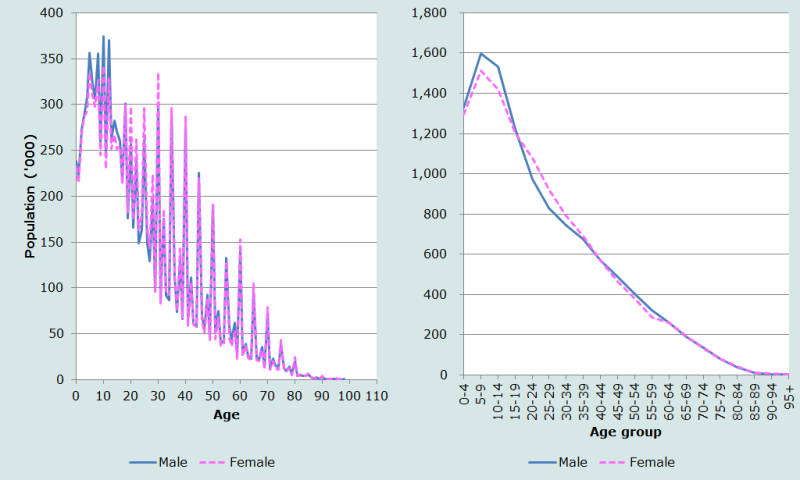
Visual inspection of the left-hand panel immediately highlights the extreme digit preference for ages ending in 0 and 5 in these data. By way of example, the population of both males and females enumerated at age 30 is more than three times the population aged either 29 or 31. Heaping is also visible on ages ending in 2 and 8. Digit preference is less marked for the population aged less than 30, although this is in part due to the heaping visible on other ages (8, 12 and 18). Clearly the reporting of individual ages is not robust in these data.
Also strongly evident in these data is the sharp fall-off in the enumerated population under the age of 5, with the enumerated population aged 1 being approximately two-thirds of that aged 5. It is unlikely that fertility has fallen by that magnitude in such a short period of time, and hence the initial presumption must be that young children were undercounted in that census. Misreporting of children’s ages – resulting in an over-statement of the number of children aged 5-9 might also have contributed to the shortfall of younger children.
Plotting the same age distribution in five-year age groups to smooth the data (right-hand panel of Figure 1) provides further insights. Again, the sharp fall-off in the population aged under 5 is visible, but visual comparison of the population aged 5-9 with that aged 10-14 suggests the possibility that there may have been some under-enumeration of children aged 5-9 too. This calls into question the possibility that there may have been large-scale transference of children aged 0-4 into the 5-9 age group. Finally, the age ratios for five-year age groups are shown in Figure 2.
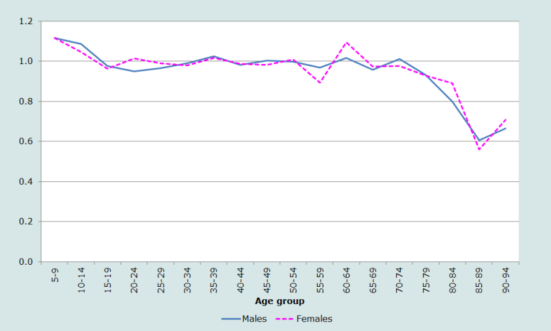
The age ratios are generally close to 1 for both sexes, except at the youngest ages (indicating some omission of children aged 0-4, as well as a lesser degree of displacement of children into the 5-9 age group). The fall-off in the age ratios at the oldest ages is to be expected given the rapid increase in mortality in those ages.
In the absence of additional information, the age and sex distributions cannot be analysed further, but the analyst may wish to compare the relevantly aged population against administrative data indicating the numbers of children enrolled in school, or compare the administratively reported births 5-9 and 10-14 years prior to the census. A comparison can also be made against the estimated population aged 5-9 derived by applying estimates of fertility rates from the mid-1990s to the estimated female population at about that time.
A second characteristic of the data that may require further investigation is the relative populations of males and females by age group. In aggregate the sex ratio of the enumerated census population is 100.5 men per 100 women. There is a noticeable surfeit of enumerated males until age 20. Between ages 20 and 40 there would appear to be more females than males. This could be the consequence of (male) labour out-migration, or a differential undercount of young adult men. The analyst should seek to find explanations for this phenomenon. However, (male) labour out-migration could plausibly account for some of the shortfall; the enumerated surfeit of men between the ages of 40 and 60 coincides with the ages at which men are most likely to return from work abroad, although this cannot account for the sex ratio rising above unity. One explanation might be that the sociological phenomena (sex-selective abortion; female infanticide) described by Sen (1992) in India might apply equally in Nepal.
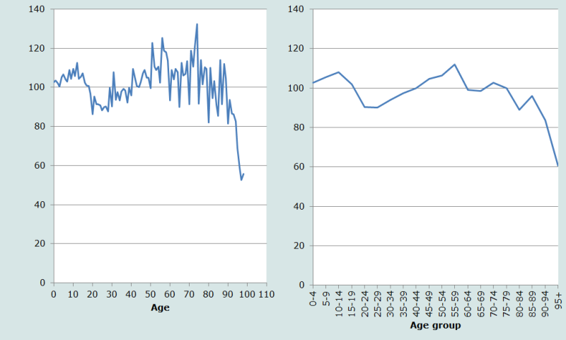
Considering Figure 3, two features of the sex ratios by single years of age (left-hand panel) stand out. First, they are quite erratic, falling sharply from age 60 onwards at ages ending in 0 and 5. This suggests that ages of men were less likely to be heaped on those digits, and more likely to be heaped for women. Second, in addition to the deficit of men between the ages of 20 and 40 identified earlier, judging from the fact that the sex ratios remain above (or very close to) unity until the oldest ages, there would also appear to be a shortage of women over the age of 40 in the census. Again, the applicability of Sen’s hypothesis to Nepal should be investigated.
The data presented by five-year age groups (right-hand panel of Figure 3) is smoother, but nonetheless reaffirms the analysis above.
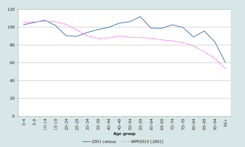
Further insights into the nature and quality of the age and sex data from the 2001 Nepal Census can be gained from a comparison of these data with the United Nations Population Division’s 2010 estimates for the country in 2001 (UN Population Division 2011). These estimates stand in marked contrast to the census data. The most effective way to show the differences is to plot the ratio of the enumerated population (by age and sex) to the UN Population Division’s estimated population for 2001 (Figure 4).
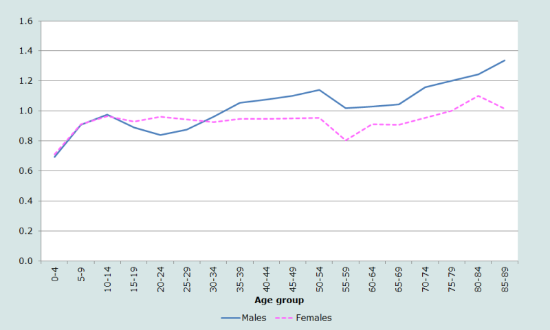
Ratios above the age of 90 are not shown as they are even more extreme – rising to 9.7 (for males) and 8.6 (for females). If they were shown, they would mask the differences at younger ages.
While the UN estimates primarily reflect the assumptions that went into them, the huge discrepancies between the two sets of estimates require careful investigation. Up until age 15, the ratios for males and females follow almost identical trends. However, the enumerated population of males and females at age 0-4 is some 30 per cent lower than that estimated by the UN, while that at 10-14 is within two or three per cent. At older ages, the patterns by sex diverge markedly: the number of women between the ages of 15 and 55 differs between the two data sources by an almost-constant five per cent.
Relative to the UN projections, there appears to be extensive age exaggeration at older ages, especially amongst men.
The comparison of the sex ratios by age calculated from the 2001 Census data, and those estimated for 2001 by the UN Population Division (Figure 5) also reveals notable differences. Further work is certainly required to understand what may account for the widely divergent accounts of the demographic structure in this country.
Checks based on multiple censuses
In addition to the checks described in the previous section, the availability of additional sets of data from earlier censuses (and vital registration systems) makes other investigations possible.
It is often difficult to determine whether irregularities revealed by the evaluation of the age and sex structure of a population in a single census are due mainly to errors in the data or to real peculiarities of the population structure. When the results of two or more successive censuses are available, it is often possible to clear up these uncertainties even without the use of any more elaborate techniques than were described in the preceding section. For example, if the age statistics from the 2008 Census of Cambodia were at hand, the possibility of explaining certain irregularities in the 1998 data as the results of birth deficits or deaths in the period of the Khmer Rouge’s rule in the late 1970s would be greatly clarified. If the 2008 figures should show the same peculiarities in the age groups ten years higher, but not in the same age groups in which they appeared in 1998, there would be a strong basis for concluding that these peculiarities reflected the true figures, rather than enumeration errors. Still more definite information regarding errors can be obtained where data from two or more censuses at intervals of a few years are available, by using balancing equations or analogous calculations with the data for particular cohorts – comparing, for example, the numbers reported at ages 10-14 in an earlier census with those reported at ages 20-24 in a census ten years later. Where data from a series of three or more censuses are available, the returns may be linked in this manner over the entire series. For the purpose of explaining the techniques, however, it is sufficient to consider examples of the use of data from two censuses.
Again, the guiding principle to be followed in comparing the results from two or more successive censuses is that population changes normally proceed in an orderly manner. When such an orderly pattern is not observed, the deviations should be explainable in terms of known events, such as the curtailment of immigration, the occurrence of famine, or some other event. Deviations from the pattern which cannot be so explained constitute a warning of possible errors; and the presumption of error is greatly strengthened if the results of other tests are found to point in the same direction. In some countries it may be possible to apply these tests to the various ethnic groups separately, if age and sex data are tabulated for such groups and if data are available on immigration and emigration of these groups (or if the groups in question are not substantially affected by international migration).
Checks making specific use of multiple censuses are, for the most part, based on (and in some cases, are) methods used to measure adult mortality – in other words, the assessment of the consistency of the data is a by-product of the methods to estimate adult mortality. This section describes some of these based on the data that are likely to be available.
Evaluation of intercensal growth rates
The growth rate, r, is defined as
where N(t1) is the total population at time t1, and similarly for N(t2).
If the country's population changes only through natural increase, it is very unlikely to have an average annual rate of growth exceeding 3.5 per cent. A rate at this level would be the result of a high birth rate (say 45 or more per 1,000) and a very low death rate (say 10 or less per 1,000). Further, it is only in unusual circumstances that the population of a developing country would be likely to decline without heavy emigration. In fact, nearly all observed rates of natural increase in modern times have been in the range from zero to 3.5 per cent. In a few developed countries, according to the 2010 World Population Prospects, natural growth is negative. If, in any given country, the rate of population change approaches or exceeds these limits without large-scale immigration or emigration, the question must be raised as to whether there is some explanation for such an unusual rate, or whether the census counts were in error.
With some information, however approximate, regarding the conditions of mortality and fertility in the country, the limits of the likely rate of growth may be defined more closely.
If population counts are available for three or more successive censuses it becomes possible to make a more accurate evaluation by comparing successive rates of growth. Again, the same principle is followed, namely, that the pattern of population growth should be regular except in so far as it can be shown that changes in the circumstances may have led to departures from the pattern.
Further, provided the censuses are undercounted to the same extent, the estimate of r is correct. Thus tracking r can provide an indication of relative undercount between pairs of data.
Cohort survival ratios
Any particular age group can be defined as a cohort: for example, boys under 5 years of age, women 50 to 54 years, or all persons 10 to 19 years of age , at a given census date. If a second census is taken exactly one decade later, the surviving members of each cohort will be exactly ten years older at the time of the second census. However, their numbers will be reduced by deaths and they may be increased or reduced by the balance of immigration and emigration. Ordinarily, mortality is the main factor; if the migration balance is negligible, the change in numbers can be used to compute a survival ratio analogous to that of a life table. Computed for one cohort only, such a survival ratio often reveals little, if anything, about the accuracy of the statistics. However, a patently absurd result would give clear evidence of error. For example, an increase in the numbers of a cohort, from one census to another, is obviously impossible, unless there has been a substantial amount of immigration. Similarly, even under conditions of very high mortality, it is unlikely that a cohort aged anywhere between 5 and 60 years at the beginning, will be reduced by one-half within a decade.
More accurate judgement is possible if the survival ratios are compared for cohorts of each sex at different ages. Survival ratios are functions of age-specific death rates, and, like these, generally conform to more or less the same pattern of variation from age to age whether mortality is high or low. The rate of survival increases after the earliest years of childhood and usually attains its maximum around age 10; thereafter it declines, at first very gradually, but more and more rapidly as advanced ages are attained. Also, at most or all ages females usually have a somewhat higher rate of survival than do males of the same age. If the hypothetical survival ratios computed for different cohorts deviate significantly from this pattern, and if no explanation (such as migration) can be found, inaccuracy in the statistics must be suspected.
Under what conditions can such comparisons of cohorts in successive censuses be made most meaningfully? One condition is either the absence of substantial net immigration or emigration or full knowledge about the age and sex composition of the migrants. A second condition, analogous to the first, is that of constant boundaries. If the country's boundaries have changed between the two censuses so that considerable numbers of people have been added to or subtracted from the population, the age and sex composition of these people must be known, if the cohort analysis is to give an accurate indication of the accuracy of the statistics. A third condition is that the population covered by the two censuses must be the same. For example, if the entire male population is enumerated in one census, but the military is excluded at the second, the age cohorts involving the military cannot be compared without a suitable adjustment, unless the number of the military is negligible. If nationals living abroad are included in one census, and excluded from another, and if the numbers involved are large, especially if they are concentrated in any particular age or sex groups, this type of analysis is invalidated.
In the case of a country where immigration is substantial, under certain circumstances a cohort can be compared at two censuses even if migration data are lacking. If the native-born population (that is to say, persons born in the country) are known not to have emigrated in significant numbers, comparisons of the two censuses can be limited to that population.
Survival ratios can be calculated over any age span and time interval, provided one has data by single years of age for at least one of the pair of censuses. With the decennial programme of censuses recommended by the United Nations, a ten-year span of ages is typical.
Method
Cohort survival ratios (CSR) measure the proportion of people enumerated at age x to x+n at time t, , in the first census, who are still alive and enumerated in a second census a years later when they are aged x+a to x+n+a at time t+a, . Thus
For graphical presentation, these estimates can be located at the mid-point of the intersurvey period (i.e. at time t+a/2) and at the midpoint of the ages at that time, x+(a+n)/2 . A plot of these cohort survival ratios offers easy and rapid insights into the quality of the data at hand, although the standard caveat still applies; a curious sequence of cohort survival ratios indicates that something may have gone amiss with the data, but does not indicate whether the fault lies with the first, the second or both censuses.
Where data from a third census are available, however, it may be that the cohort survival rates derived from the first two censuses appear reasonable, while those derived from the second and third appear problematic. In this case, one would proceed by assuming that the fault lies with the enumeration in the third census, and not the second.
Finally, if one has an appropriate life table at one’s disposal, one could derive a further ratio by dividing the Cohort Survival Ratio into the equivalent ratio implied by the life table, resulting in a ratio of ratios at each age
If the census suffered no error, the age structure of the enumerated population was identical to that described by the life table, and the mortality experience was exactly that indicated by the life table (all three strong conditions), the ratio would take the value of 1. Departures from unity would indicate either error in the data, or an inappropriate choice of life table. Further, under these conditions and in the absence of migration, ratios less than unity would imply an under-enumeration in the second census relative to the first and vice versa.
Example
Censuses in Zimbabwe were conducted exactly 10 years apart (the official Census date being 18 August) in 1982, 1992 and 2002. Tabulations of the enumerated population by age and sex are available from the Demographic Yearbooks on the UN Statistics Division Website (the 1997 Historical Supplement and the 2008 Yearbook were used). The tabulations are shown in Table 1. The data present the population aged under 1 and aged 1-4 separately; these populations are kept distinct for the purpose of more accurately understanding the population dynamics given the rapid changes in mortality in the first few years of life.
Table 1 Population of Zimbabwe by age and sex, 1982, 1992 and 2000 Censuses
1982 | 1992 | 2002 | ||||||
|---|---|---|---|---|---|---|---|---|
Age | Male | Female | Male | Female | Male | Female | ||
0 | 133,070 | 136,960 | 167,552 | 169,064 | 170,054 | 170,277 | ||
1-4 | 510,260 | 528,390 | 621,411 | 626,664 | 668,008 | 667,730 | ||
5-9 | 612,760 | 619,300 | 821,319 | 832,469 | 764,453 | 769,247 | ||
10-14 | 529,750 | 518,740 | 724,905 | 731,846 | 754,587 | 757,657 | ||
15-19 | 390,160 | 412,610 | 615,728 | 632,510 | 736,686 | 766,890 | ||
20-24 | 290,380 | 364,200 | 466,837 | 523,060 | 564,034 | 658,873 | ||
25-29 | 243,420 | 281,060 | 335,713 | 376,495 | 473,984 | 513,793 | ||
30-34 | 185,400 | 206,760 | 280,066 | 326,299 | 369,836 | 360,291 | ||
35-39 | 147,920 | 170,170 | 229,360 | 259,555 | 235,692 | 268,797 | ||
40-44 | 142,050 | 139,530 | 174,266 | 189,509 | 194,702 | 239,727 | ||
45-49 | 116,490 | 110,390 | 145,437 | 143,441 | 165,437 | 191,168 | ||
50-54 | 111,780 | 90,880 | 133,261 | 147,339 | 128,029 | 173,229 | ||
55-59 | 67,400 | 60,800 | 94,713 | 86,729 | 98,417 | 112,498 | ||
60-64 | 76,850 | 65,260 | 95,510 | 84,213 | 94,447 | 99,420 | ||
65-69 | 38,810 | 38,860 | 51,202 | 50,902 | 64,301 | 67,851 | ||
70-74 | 29,810 | 30,500 | 58,279 | 62,479 | 60,311 | 62,464 | ||
75+ | 39,410 | 46,760 | 52,026 | 68,403 | 71,950 | 92,311 | ||
Unknown | 7,900 | 6,680 | 15,952 | 18,034 | 19,252 | 25,254 | ||
Total | 3,673,620 | 3,827,850 | 5,083,537 | 5,329,011 | 5,634,180 | 5,997,477 | ||
Provided there are no grounds for believing that records with missing ages are not concentrated disproportionately in certain age groups, the first step is to apportion the (proportionately relatively small) number of cases where age is missing in proportion to the population size in each age group from 0 to 75+. In the 1982 Census, the proportion of the population with unknown age was 0.19 per cent; this doubled to 0.38 per cent in the 2002 Census. The resulting distributions are shown in Table 2.
Table 2 Adjusted population of Zimbabwe by age and sex, 1982, 1992 and 2002 Censuses
1982 | 1992 | 2002 | ||||||
|---|---|---|---|---|---|---|---|---|
Age | Male | Female | Male | Female | Male | Female | ||
0 | 133,357 | 137,199 | 168,079 | 169,638 | 170,637 | 170,997 | ||
1-4 | 511,360 | 529,314 | 623,367 | 628,792 | 670,298 | 670,554 | ||
5-9 | 614,081 | 620,383 | 823,904 | 835,296 | 767,074 | 772,500 | ||
10-14 | 530,892 | 519,647 | 727,187 | 734,331 | 757,174 | 760,861 | ||
15-19 | 391,001 | 413,331 | 617,666 | 634,658 | 739,212 | 770,133 | ||
20-24 | 291,006 | 364,837 | 468,307 | 524,836 | 565,968 | 661,659 | ||
25-29 | 243,945 | 281,551 | 336,770 | 377,773 | 475,609 | 515,966 | ||
30-34 | 185,800 | 207,121 | 280,948 | 327,407 | 371,104 | 361,815 | ||
35-39 | 148,239 | 170,467 | 230,082 | 260,436 | 236,500 | 269,934 | ||
40-44 | 142,356 | 139,774 | 174,815 | 190,152 | 195,370 | 240,741 | ||
45-49 | 116,741 | 110,583 | 145,895 | 143,928 | 166,004 | 191,976 | ||
50-54 | 112,021 | 91,039 | 133,680 | 147,839 | 128,468 | 173,962 | ||
55-59 | 67,545 | 60,906 | 95,011 | 87,023 | 98,754 | 112,974 | ||
60-64 | 77,016 | 65,374 | 95,811 | 84,499 | 94,771 | 99,840 | ||
65-69 | 38,894 | 38,928 | 51,363 | 51,075 | 64,521 | 68,138 | ||
70-74 | 29,874 | 30,553 | 58,462 | 62,691 | 60,518 | 62,728 | ||
75+ | 39,495 | 46,842 | 52,190 | 68,635 | 72,197 | 92,701 | ||
Unknown |
|
|
|
|
|
|
|
|
Total | 3,673,620 | 3,827,850 | 5,083,537 | 5,329,011 | 5,634,180 | 5,997,477 | ||
In keeping with the principles outlined earlier, the basic age and sex characteristics of the population are investigated first. The unavailability of data by single years of age means that this aspect of the data quality cannot be investigated. The age and sex distributions of the Zimbabwean population from the three censuses are shown in Figure 6.
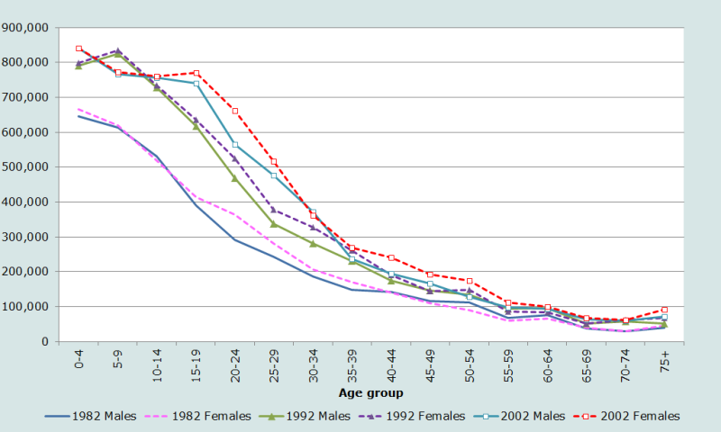
In all three censuses there is a clear surfeit of women between the ages of 15 and (at least) 35. This is almost certainly a product of labour migration of young men to neighbouring countries, most obviously South Africa. There would appear to have been a sizeable underenumeration of the population under the age of 5 in the 1992 Census – the population in that age group is less than that then aged 5-9, unlike the adjacent censuses.
Age and sex ratios from the three censuses are shown in Figure 7.
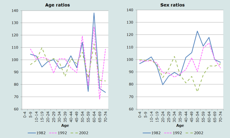
The age ratios in the 60-64 age group are particularly high in all three censuses, and the excess population at that age contributes to the very low age ratios in the 55-59 and 65-69 age groups. The sex ratios start off close to 100, and fall rapidly after age 15 in each census, probably indicating migration of young men. Of greater concern is the rise in the sex ratios between ages 35 and 55 to levels far in excess of 100 in the 1982 Census. This almost certainly reflects some undercount of women. Sex ratios at the oldest ages are still very high, probably reflecting age exaggeration among older men.
The highly erratic age and sex ratios do not inspire a great deal of confidence in the quality of the data.
Next, cohort survival rates are derived as above, for each sex separately since patterns and level of mortality differ for males and females. Since the population aged 0-4 in 1992, for example, would be aged 10-14 in 2002, we assume that the survival rate for this cohort applies (roughly) to people aged 7½ at the midpoint between the censuses in August 1997. Cohort survival rates are not estimated for the very young, or for the open interval. The results are presented graphically in Figure 8.
The top left panel shows the cohort survival rates between the 1982 and 1992 Censuses by sex; the bottom left panel shows the equivalent data from the 1992 and 2002 Censuses. There was an evident undercount of children of both sexes as well as women up until around the age of 20 in the 1982 Census (or, improbably, high levels of child in-migration between 1982 and 1992), as indicated by the survival ratios greater than one.
While both left-hand panels show (broadly) a pattern of decreasing survival ratios (increasing mortality) by age, the data are far from consistent either by sex or by age. It is unlikely, for example, that the survival ratios for men will be greater than those for women of the same age. There is also a very curious spike in both intercensal periods in the survival ratios of women aged 40-44 in first period to 50-54 in the next. This should be investigated further.
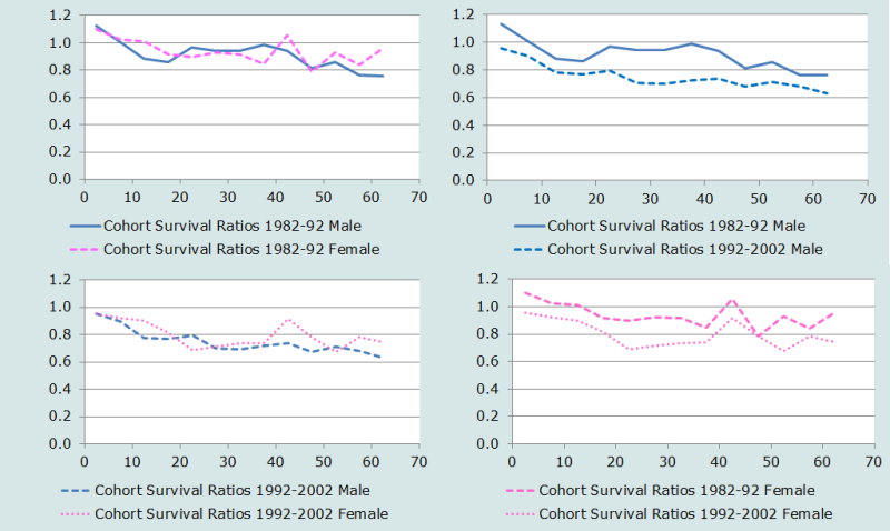
The two right-hand panels depict the cohort survival ratios over time, for men and women separately. They indicate a pattern of substantially increased mortality in Zimbabwe over the two ten-year periods. While the erratic nature of the survival ratios indicates the relatively poor quality of the data, this increase is almost certainly attributable largely to the effect of HIV/AIDS among adults in the country in the second period, in conjunction with the rapidly worsened socio-economic conditions that prevailed in the country towards the turn of the century, which almost certainly fuelled extensive out-migration of younger adults. The apparent increase in mortality among children and young adults seen in the two right-hand panels is almost certainly largely attributable to the poor enumeration of this population in 1982.
Post-enumeration surveys
A post-enumeration survey (PES) uses the logic of capture-recapture techniques to estimate the proportion of the population that was not enumerated at the time of the census. This is done by returning to sample sites to readminister a second, short, questionnaire to all households which should have been enumerated in that site, after which households and individuals captured in this survey are matched, wherever possible, with those from the census. This procedure should give a concrete estimate of the magnitude of the undercount which can be compared to and contrasted with that implied by, for example, an analytical population projection. The results from the PES, then, can be used to scale up (“weight”) the enumerated data to compensate for the undercount.
A PES is thus potentially extremely useful. However, the two key assumptions underlying the use of capture-recapture techniques are that the probabilities of being found in the census and the PES are independent of each other; and that it is possible to identify the same individual unambiguously in both data sets. The first assumption is unlikely to hold in human populations - certain groups who avoid being counted in a census (illegal immigrants, for example), are likely also to avoid a PES. In this sense, the PES gives information only on those known to have been missed in the census; it tells nothing of those not known to have been missed. The second assumption is also unlikely to hold, particularly in settings with high population mobility or if the interval between the census and the PES is long.
The principles and best practice associated with the conduct of a PES are documented in a 2010 manual (UN Statistics Division 2010).
Where a PES is conducted, ideally the analyst will have access to the report on the PES so as to understand any deficiencies in that study. The ability of the PES to provide finely-grained insights into the data collected in the census is directly related to the size of the PES as well as to the delay between the census date and the date of the PES. Given the time and cost constraints, the sample size of a PES is typically much smaller than a full census. Accordingly estimates of an undercount have to be made at a fairly coarse level. Thus, for example, in the 2001 South African Census, the estimates of the undercount were made using only broad age groups, sex, population group, province, and enumerator area geo-type (urban, rural, formal, informal). In turn, this means that the population is assumed to be equally undercounted within each group defined by the five characteristics above. Hence, at granularities finer than those used to determine the undercount, the resulting estimate of the count may not be reliable.
Insights into the magnitude of the adjustments made, and the extent of the undercount, can be gained from an evaluation of the weights provided with the data. If the raw data made available from a census are unadjusted by a PES, then the data weights will reflect the sampling fraction: in a random 10 per cent sample drawn from a full census, each record would be deemed to be representative of 10 people, and hence carry a weight of 10. Where a PES has been conducted, the excess of the weight over the sampling fraction reveals the undercount. Analytically,
Hence, if for a particular record, the weight is 11.8 in a ten per cent sample (i.e. a sample fraction of 0.1), this implies an adjustment in respect of an undercount of 15.3 per cent (1- (1/0.1)/11.8).
Where estimates of the undercount have not been provided with the data, applying this last formulat to the weights provided to different groups within the population allows the analyst to reverse-engineer the estimated undercounts to a fairly high degree of accuracy.
References
Feeney G. 2003. "Data assessment," in Demeny, P and G McNicoll (eds). Encyclopaedia of Population. Vol. 1. New York: Macmillan Reference USA, pp. 190-193.
Garenne M. 2004. "Sex ratios at birth in populations of Eastern and Southern Africa", Southern African Journal of Demography 9(1):91-96. https://www.jstor.org/stable/20853265
Minnesota Population Center. 2015. Integrated Public Use Microdata Series, International. Version 6.4 [Machine-readable database]. Minneapolis, MN: University of Minnesota. https://doi.org/10.18128/D020.V6.4
National Research Council. 2004. The 2000 Census: Counting under Adversity. Panel to Review the 2000 Census. Citro, Constance F., Daniel L. Cork and Janet L. Norwood (eds), Committee on National Statistics, Division of Behavioural and Social Sciences and Education. Washington DC: National Academies Press.
Sen A. 1992. "Missing women", British Medical Journal 304(6827):587-588. doi: https://dx.doi.org/10.1136/bmj.304.6827.587
Shryock HS and JS Siegel. 1976. The Methods and Materials of Demography (Condensed Edition). San Diego: Academic Press.
UN Population Branch. 1955. Manual II: Methods of Appraisal of Quality of Basic Data for Population Estimates. New York: United Nations, Department of Economic and Social Affairs, ST/SOA/Series A/23. https://www.un.org/development/desa/pd/sites/www.un.org.development.desa.pd/files/files/documents/2020/Jan/un_1955_manual_ii_-_methods_of_appraisal_of_quality_of_basic_data_for_population_estimates_0.pdf
UN Statistics Divison. 2008. Principles and Recommendations for Population and Housing Censuses v.2. New York: Department of Economic and Social Affairs, ST/ESA/STAT/SER.M/67/Rev.2.
https://unstats.un.org/unsd//demographic/sources/census/docs/P&R_%20Rev2.pdf
United Nations. 2020. Handbook on Population and Housing Census Editing, Revision 2. New York: United Nations, Department of Economic and Social Affairs, ST/ESA/STAT/SER.F/82/Rev.1.
https://unstats.un.org/unsd/publication/SeriesF/seriesf_82rev2e.pdf
United Nations. 2010. Post-Enumeration Surveys: Operational Guidelines - Technical Report. New York: United Nations, Department of Economic and Social Affairs.
https://unstats.un.org/unsd/demographic/standmeth/handbooks/Manual_PESen.pdf
UN Population Division. 2011. World Population Prospects: The 2010 Revision, Volume I: Comprehensive Tables. New York: United Nations, Department of Economic and Social Affairs, ST/ESA/SER.A/313.
https://population.un.org/wpp/Publications/Files/WPP2012_Volume-I_Comprehensive-Tables.pdf
US Bureau of the Census. 1985. Evaluating Censuses of Population and Housing. Statistical Training Document ISP-TR-5. Washington, DC: US Bureau of the Census.
https://www.census.gov/library/working-papers/1985/adrm/rr85-24.html
US Census Bureau. 1997. Population Analysis Spreadsheets for Excel. Washington, DC: US Bureau of the Census. https://www.census.gov/data/software/pas.html
- Printer-friendly version
- Log in to post comments