Introduction to model life tables | Tools for Demographic Estimation

Use of model life tables in mortality estimation

Model life tables are used for comparison in the assessment of empirical estimates of mortality, to smooth or otherwise adjust defective mortality estimates, and to complete the life table when estimates of mortality are available for only a limited range of ages.

The term "to smooth" in this context refers to any procedure for the elimination or minimization of irregularities present in reported data or in preliminary estimates obtained from them. Such smoothing techniques encompass a wide variety of procedures ranging from the fitting of models to simple averaging. Traditional techniques for the smoothing or graduation of age distributions and observed age-specific mortality rates such as the use of cubic splines are well described in the actuarial and demographic literature and are not discussed here. Instead, the focus is on model-based procedures that are suitable for use when the basic data are either defective or incomplete.

In classical demographic analysis, a life table is calculated by converting a complete series of age-specific death rates (_nm_x) into probabilities of dying (_nq_x). From these one can calculate survivorship, l(x), and all the other functions of the life table. In the analysis of census and survey data, however, one often only obtains mortality estimates for part of the age range. For example, mortality estimates made from birth history data and sibling history data provide no information on the mortality of older children or on adult mortality at age 50 and more. With estimates of this sort, model life tables can be used both to smooth the estimated death rates and to complete the life table by making plausible assumptions about the death rates that prevail at ages at which mortality has not been measured directly.

Furthermore, if one has estimated survivorship indirectly from information on children ever born and surviving and on the survival of parents or other adult relatives, the results indicate only the level of mortality in each broad age range. In particular, for adults these methods yield conditional survivorship probabilities i.e. probabilities of surviving from age A to age B, l(B)/l(A). In this situation, model life tables can be used both to estimate death rates for five-year age groups and to complete the life table by making a plausible assumption about mortality in old age.

The following two chapters describe two approaches to deriving complete life tables from information on mortality in a limited range of ages. Chapter 32 focuses on methods for combining a single estimate of child mortality (₅q₀) and a conditional estimate of adult mortality referring to the same year or period of years to derive a full life table. Several variants of the method are described. Chapter 33 describes a method for combining a series of time-located estimates of child mortality (such as those produced indirectly from data on children ever-born and surviving) and a series of time-located estimates of conditional adult survival (such as those produced by the indirect orphanhood or siblinghood methods) to produce a life table for a specific point in time.

This manual makes extensive use of relational logit model life tables, firstly, for the evaluation and smoothing of series of estimates of child and adult mortality and, secondly, to combine independent estimates of child and adult mortality and produce full life tables. The system and its properties are described in the next section.

Overview of the relational logit system of model life tables

Brass and colleagues (Brass 1964, 1971; Brass and Coale 1968) developed a flexible 2-parameter system of model life tables usually referred to as the logit model life table system. Broadly speaking, the first parameter of this system of models, α, captures differences in the level of mortality between populations and the second parameter, β, variation between populations in the relationship between mortality in childhood and adulthood.

The system of models is a relational one. In other words, it is based on a mathematical transformation of the age-specific survivorship function, l(x), which makes it possible to relate two different life tables to each other by means of a simple equation. In particular, Brass discovered that a logit transformation of the probabilities of survival to age x, l(x), rendered the relationship between transformed probabilities for different life tables approximately linear.

Thus, if one defines the logit of l(x) as

$Y (x) = logit (l (x)) = - \frac{1}{2} \ln (\frac{l (x)}{1 - l (x)}),$

the following linear relationship is approximately true for all ages x:

$Y (x) = α + β Y^{*} (x),$

where Y (x) and Y^*(x) are the logits of survivorship by age, l(x) and l^*(x), in two different life tables, and α and β are constants.

Those familiar with logistic regression will recognize Y(x) as being half the log odds of dying between birth and age x since

$logit (l (x)) \times 2 = - \ln (\frac{l (x)}{1 - l (x)}) = \ln (\frac{1 - l (x)}{l (x)}) = \ln (\frac{{}_{x}q_{0}}{1 - {}_{x}q_{0}}) .$

If Equation 2 held for any pair of life tables, this would imply that all life tables could be generated from a single baseline or standard life table, l^s(x), using an appropriate pair of values of α and β. In fact, Equation 2 is only approximately satisfied by pairs of actual life tables, but the approximation is close enough to warrant use of the relationship to study and model observed mortality schedules.

Before describing how to use Equation 2 to generate model life tables, a word about the meaning of the parameters α and β is in order. Consider the set of life tables that can be generated starting with some baseline life table l^s(x) and calculating Y(x) for different values of α and β. If β is held constant and equal to 1, changing α will either increase or decrease survivorship at every age. Thus changing α will produce life tables whose shapes are essentially the same as that of the l^s(x) life table used to generate them, but whose overall levels differ. If, on the other hand, α is fixed at 0 and β is allowed to vary, the resulting life tables will no longer display the same shape as l^s(x). All of the derived tables will intersect at a single point located somewhere in the central portion of the age range, where l^s(x) = 0.5 and Y^s(x) = 0. Therefore, their probabilities of survival will be either lower at younger ages and higher at older ages or lower at younger ages and higher at the older than the standard survivorship probabilities l^s(x) from which they are generated. Hence, β modifies the shape of the generated mortality schedule rather than its level. Simultaneous changes of α and β will bring about changes in both the level and shape of the survivorship function being generated.

From Equation 1,

$l (x) = \frac{1}{1 + \exp (- 2 Y (x))}$

and combining this with Equation 2:

$l (x) = \frac{1}{1 + \exp (- 2 (α + β Y^{s} (x)))} .$

Thus, for any series of l^s(x) values defining a standard life table, another series l(x) can be obtained for each pair of α and β values. (Note that, at the endpoints of the age range, Equation 3 cannot be used to calculate l(x); l(0) and l(ω) should be set to 1 and to 0, respectively).

Equation 3 can be used to generate families of model life tables from an appropriate standard life table, l^s(x). Potentially, any life table can be used as a standard. For example, one might use a reliable life table for the population concerned at some other date or a life table from a neighbouring country. When no appropriate or reliable such life table exists, however, a model life table taken from the Princeton regional series (Coale, Demeny and Vaughan 1983), or the UN Model Life Tables for Developing Countries (UN Population Division 1982) is frequently used as a standard. The derivation of the standards used in this Manual are described in the next section of this chapter.

Because of the mathematical simplicity of Equations 2 and 3, logit model life tables based on any standard can be readily calculated in a spreadsheet, doing away with the need for volumes of published tables. The simple mathematical form of Equation 3 also simplifies the use of relational logit model life tables for simulation purposes and for projecting mortality. If the past and current mortality schedules of a population are known, trends in the α and β parameters can be determined by using the logit model life table system to fit each mortality schedule, and with some caution the trends in these two parameters can be projected to generate estimates of future mortality.

Description of the model life tables used in the Manual

All the logit life tables used in this manual are based on a common set of standard life tables. These standard life tables are taken from the Princeton regional model life tables (North, South, East and West) and the UN model life tables for developing countries (General, Latin American, Chilean, South Asian, Far Eastern), by sex. They all have an expectation of life at birth of 60 years. The original life tables have been modified, extended and enhanced over time to extend them to older ages. We make use of these updated tables, which were developed for the population projections in the World Population Prospects 2012 (UN Population Division 2013). These life tables provide values of l(x) and L_x (amongst other quantities) for ages 0, 1, 5, 10, ..., 130.

For the standards based on the Princeton regional model life tables, values for l(2), l(3) and l(4) were generated by applying the proportionality factors presented by Coale, Demeny and Vaughan (1983: 21) to l(1) and l(5). For the standards based on the UN Model Life Tables for Developing Countries, deaths between the ages of 1 and 5 were distributed by single years of age in the same proportion as those deaths in the original sex-and region-specific life tables (UN Population Division 1982).

Some methods of child and adult mortality estimation require joint-sex life tables (that is, life tables for males and females combined). As these life tables (or their implementation) are not particularly sensitive to the sex ratio at birth, a sex ratio at birth of 105 (boys per 100 girls) is used. Joint-sex life tables were then derived by appropriate weighting of the sex-specific life tables:

$l^{c} (x) = \frac{(1.05) l^{m} (x) + l^{f} (x)}{2.05}$

where l^c(x) represents the number of survivors at age x in the joint-sex life table and l^m(x) and l^f(x) are the equivalent life table values for men and women respectively.

As these life tables are used almost exclusively in a relational context (as originally set out by Brass (1971), standard logits of the l^s(x) values were calculated for all ages above zero by means of the formula

$Y^{s} (x) = 0.5 \ln (\frac{1 - l^{s} (x)}{l^{s} (x)}) .$

Values of these logits can be downloaded from the Tools and resources page.

Choosing an appropriate standard

A crucial decision to be made when implementing methods based on model life tables, or when combining estimates from different methods into a single life table based on the relational model life table system is the choice of standard life table to be used in the calculations.

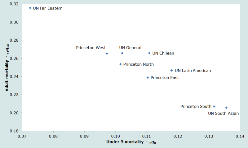
The nine standard life tables (four Princeton regional model life tables; five UN developing country life tables) used in this manual exhibit markedly different mortality patterns. Figure 1 shows the relative balance of child and adult mortality for the combined sex standard life tables – all of which have a life expectancy at birth of 60 years. The index of child mortality is ₅q₀, the probability of dying before exact age 5; the index of adult mortality is ₄₅q₁₅, the conditional probability of dying between exact ages 15 and 60.

Thus, for example, the UN Far Eastern table is revealed to have very high adult mortality and very low child mortality relative to the other tables used, while – at the other extreme – the Princeton South and UN South Asian tables have relatively low adult mortality but very high child mortality.

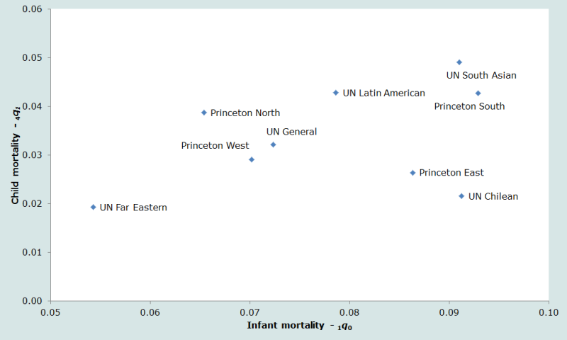
A second important dimension on which the tables differ is in the balance between infant mortality (before the first birthday) and child mortality (between exact ages 1 and 5). Comparing these rates (Figure 2), it can be seen that while the UN Far Eastern and UN Chilean tables have roughly equivalent levels of child mortality, the level of infant mortality in the two standards is very different.

Figure 1 Relationship between adult and under five mortality for different standard life tables with a life expectancy at birth of 60 years

Figure 2 Relationship between infant and child mortality for different standard life tables with a life expectancy at birth of 60 years

Ideally, a standard life table should be selected for any application that describes well the relative balance between infant and child mortality, on the one hand, and between under five mortality and adult mortality on the other. Thus, if there are reasonable estimates of the mortality pattern for a given country, the best standard life table can be selected by comparing the observed pattern to those embodied by the model tables. But in populations on which little or no reliable information on mortality by age is available, the analyst can do little more than guess which pattern would be most appropriate.

In situations where nothing is known about the age pattern of mortality, use of either the Princeton West or the UN General standard is recommended because of the relatively wide data base from which these tables were derived. Moreover, the UN General pattern, in particular, appears to represent something close to an average pattern in terms of characteristics plotted in Figures 1 and 2.

As for the "extra information" that might permit a more enlightened selection, it can vary considerably in type and quality. It might range, for example, from estimates of age-specific mortality rates derived from vital registration data to knowledge of some fairly general facts, such as the prevalence and typical duration of breast-feeding in the population, or an estimate of tuberculosis prevalence.

When a set of observed age-specific mortality rates is available (preferably a set adjusted according to a death distribution method such as those described in Chapters 24 and 25), a model mortality pattern may be chosen by comparing the logits of the observed l(x) values to those in the different standard model life tables. This comparison may be carried out by plotting the observed values of Y(x) against those derived from the different standards, and choosing as the preferred standard that model life table that exhibits the most linear relationship between the two sets of values.

According to the description given above of the mortality patterns contained in the different standard life tables, it is evident that they differ most markedly in their values at early ages and in the relation between infant (₁q₀) and child (₄q₁) mortality. It follows that quite different child mortality estimates may be obtained from the same information according to which family is selected as representative. Furthermore, in this case, sound external evidence to inform the selection of a standard can be hard to obtain, mainly because infant deaths are very often grossly underreported. In the absence of adequate empirical data for selecting a suitable standard life table, a few general guidelines can be proposed to help narrow the possibilities and lead to a reasonable choice:

(a) In a population where breast-feeding is common practice and where weaning occurs at a relatively late age (12 months or over), one may reasonably expect child mortality (₄q₁) to be relatively high compared with infant mortality (₁q₀) since breast-feeding may successfully prevent deaths due to malnutrition and infectious diseases among young infants. When weaning takes place, however, the child is less protected from these perils and is more likely to die. In these cases, mortality in childhood is likely to be well represented by the Princeton North or UN General standard. Yet, it cannot be inferred from these observations that these tables will provide an appropriate mortality model for other sections of the age range. Only independent information on mortality in adulthood is able to establish this fact;

(b) In some populations today, breast-feeding has been abandoned by a high proportion of the female population; and, from a very early age, infants are fed unsterilized and often inadequate rations of "milk formula". When this practice is adopted by women living in relatively unhealthy conditions and exacerbated by poor care at delivery and immediately after birth (perhaps leading to a high incidence of neonatal tetanus), infant mortality can be high relative to mortality later in childhood. In such conditions, the Princeton East or UN Chilean tables may be a good representation of mortality in childhood. The caution in the previous paragraph about whether these tables may adequately describe the balance between adult and child mortality applies;

(c) Early weaning may not be the only cause of malnutrition which results in a high infant and child mortality. In some populations, breast-feeding is nearly universal but both levels of hygiene and children’s nutritional status are poor and both infant and child mortality are high. For such least developed countries, either the Princeton South or UN South Asian model life tables may be the most appropriate;

(d) In the absence of data adequate to determine the most suitable family of model life tables to use for a particular country, one may select the same family as that employed for a neighbouring country with similar cultural and socio-economic characteristics;

(e) For the reasons given earlier, if little is known about the population under study, the Princeton West or UN General standard is recommended.

From these remarks, it is clear that the knowledge about mortality patterns is still fairly limited and that, certainly, better information concerning the mortality experience of populations in developing countries is needed to assess the adequacy of the models now available.

Alternative systems of model life tables

Two of the methods of fitting life tables to observed data presented in the next chapter make use of two somewhat different approaches to the modelling of mortality patterns to that pioneered by Brass. These two alternative systems of model life tables are described briefly below. The interested reader is referred to the source texts for further information.

The modified logit system

Murray and colleagues (Murray, Ferguson, Lopez et al. 2003) proposed a modified system of relational logit model life tables based on a single global standard life table and an additional two sets of age-specific coefficients γ(x) and θ(x):

$Y (x) = α + β Y^{s} (x) + γ (x) (1 - (\frac{l (5)}{l^{s} (5)})) + θ (x) (1 - (\frac{l (60)}{l^{s} (60)})) .$

As before, Y(x) denotes the logit transform of l(x), so the first two elements are those of the Brass system of logit model life tables. The first of the two additional sets of coefficients, γ(x), adjusts for the level of under-five survivorship relative to the standard, while θ(x) does the same for the level of adult survivorship relative to the standard.

Despite superficially appearing to be a 4-parameter model, this modification of the logit system of models actually remains a 2-parameter one. Because γ(5), θ(5), γ(60) and θ(60) are all set to zero by definition, α and β fully define l(5) and l(60) in the fitted model and, thereby, the two sets of age-specific deviations from the standard pattern of mortality, γ(x) and θ(x). In effect, these deviations serve to reduce the impact on mortality in infancy and old-age of using a value of β other than 1 to model the relationship between mortality in childhood and adulthood as a whole.

Users of this system of models should be alert to the fact that the values of γ(x) and θ(x) published in the 2003 paper are reversed with respect to sign. Therefore, the parameters tabulated in Table 3 of that paper should be multiplied by -1 before using them.

The log quadratic system

An alternative 2-parameter system of model life tables has been published recently by Wilmoth, Zureick, Canudas-Romo et al. (2012). It uses age-specific scalar constants a(x), b(x), c(x) and v(x) and parameters h and k in the following relationship:

$\ln (_{n} m_{x}) = a (x) + b (x) h + c (x) h^{2} + v (x) k .$

Values of a(x), b(x), c(x) and v(x) were derived from the mortality data contained in the Human Mortality Database, leaving two parameters (h and k) with which to fit the model to empirical estimates of mortality.

The first parameter, h, measures the overall level of mortality and is defined as the log of the observed ₅q₀. The second parameter k (in combination with v(x)) captures the deviation of the observed age pattern of mortality from that of a standard population. In practice, it is chosen to fit one index or a series of observed indices of adult mortality (e.g. ₄₅q₁₅ or ₃₀q₃₀).

References

Brass W. 1964. Uses of census or survey data for the estimation of vital rates. Paper prepared for the African Seminar on Vital Statistics, Addis Ababa 14-19 December 1964. Document No. E/CN.14/CAS.4/V57. New York: United Nations.

Brass W. 1971. "On the scale of mortality," in Brass, W (ed). Biological Aspects of Demography. London: Taylor and Francis, pp. 69-110.

Brass W and AJ Coale. 1968. "Methods of analysis and estimation," in Brass, W, AJ Coale, P Demeny, DF Heisel, et al. (eds). The Demography of Tropical Africa. Princeton NJ: Princeton University Press, pp. 88-139.

Coale AJ, P Demeny and B Vaughan. 1983. Regional Model Life Tables and Stable Populations. New York: Academic Press.

Murray CJ, BD Ferguson, AD Lopez, M Guillot, J Salomon and O Ahmad. 2003. "Modified logit life table system: principles, empirical validation, and application", Population Studies 57(2):165-182. doi: https://dx.doi.org/10.1080/0032472032000097083

UN Population Division. 1982. Model Life Tables for Developing Countries. New York: United Nations, Department of Economic and Social Affairs, ST/ESA/SER.A/77. https://www.un.org/development/desa/pd/sites/www.un.org.development.desa.pd/files/files/documents/2020/Jan/un_1982_model_life_tables_for_developing_countries.pdf

UN Population Division. 2011. Model Life Tables. New York: United Nations, Department of Economic and Social Affairs. https://www.un.org/development/desa/pd/data/model-life-tables

UN Population Division. 2013. World Population Prospects: The 2012 Revision. New York: United Nations, Department of Economic and Social Affairs. https://www.un.org/development/desa/pd/sites/www.un.org.development.desa.pd/files/files/documents/2020/Jan/un_2012_world_population_prospects-2012_revision_highlights.pdf

Wilmoth JR, S Zureick, V Canudas-Romo, M Inoue and C Sawyer. 2012. "A flexible two-dimensional mortality model for use in indirect estimation", Population Studies 66(1):1-28. doi: https://dx.doi.org/10.1080/00324728.2011.611411

Author

Moultrie TA and IM Timæus

Printer-friendly version
Log in or register to post comments

Suggested citation

Moultrie TA and IM Timæus. 2013. Introduction to model life tables . In Moultrie TA and IM Timæus (eds). Tools for Demographic Estimation. Paris: International Union for the Scientific Study of Population. https://demographicestimation.iussp.org/content/introduction-model-life-tables. Accessed 2024-04-20.