Indirect estimation of child mortality
Description of the method
Indirect methods, pioneered by Brass and Coale (1968), estimate child mortality from information on aggregate numbers of children ever born and children still alive (or dead) reported by women classified by age group (or alternatively grouped by time since first birth, or marital duration).
Such information is described as a summary birth history (SBH). The amount of detail collected varies, from just two questions (number of children ever born and number of children still alive) to the most detailed SBH asking separately about boys and girls, and enquiring separately about surviving children living at home versus those living elsewhere described in the introduction to child mortality analysis as part of the DHS full birth history sequence of questions. The proportion dead of children born to women by age (or time since first birth, or duration of marriage) reflects the level of child mortality, but is also affected by other things, primarily the age pattern of childbearing and the age pattern of child mortality. Young mothers generally have young children, who have been exposed to the risk of death for short, recent periods; the proportion dead for such mothers thus reflects child mortality risks to an early age. Older mothers, in contrast, have a mix of young and older children exposed to the risk of dying for longer periods on average further in the past. Through models of fertility and child mortality, the proportions dead are converted into probabilities of dying by exact ages of childhood, nq0. The older the women, the greater the value of n.
If mortality has changed over time, the estimated probabilities of dying reflect the mortality rates that have prevailed at a range of ages and dates. Fortunately, a `time location’ method has been developed that estimates how many years previously each proportion dead approximates period probabilities of dying. These intervals increase with the age of respondents. Thus, if the probabilities of dying estimated from the reports of different age groups of woman are translated into a common index of mortality, these statistics will refer to different dates and can be used to infer the broad trend in mortality over time.
Data requirements and assumptions
Tabulations of data required
- Number of women, grouped by five-year age, duration of marriage, or time since first birth.
- Number of children ever born alive by women by relevant (age, time since first birth, or marriage duration) five-year group.
- Number of children born alive by the women that have died before (or are still alive at) the time of the survey, by relevant five-year group.
- Number of births in the year before the survey by five-year age group (optional).
Important assumptions
- Population age patterns of fertility and child mortality are adequately represented by the model patterns used in developing the method.
- In any time period, mortality of children does not vary by five-year grouping of mothers.
- No correlation exists between mortality risks of children and survival of mothers (by mortality or migration) in the population (see effects of HIV on methods of child mortality estimation).
- Any changes in child mortality in the recent past have been gradual and unidirectional.
- Cross-sectional average numbers of children ever born by age (or by duration of marriage or time since first birth) adequately reflect the appropriately-defined cohort patterns of childbearing.
Preparatory work and preliminary investigations
Data quality assessment for an SBH involves a subset of analyses described under the section on direct estimation of child mortality for the analysis of a full birth history (FBH). Since an SBH contains no information on dates of individual births, assessment is limited to analysis of aggregates, tabulated by age group of mother (or duration of marriage or time since first birth, if such information is available); single-year tabulations can also be revealing if there is substantial age heaping. Once again, assessments are carried out of internal plausibility within the data set itself, and of external consistency with other data sets for the population. Of internal assessments, a first check should be of the average number of children ever born (CEB) in each group of women. (Note that the appropriate denominator for these calculations is all women, not the number of mothers or number of ever-married women). Unless fertility has been rising, the average number of CEB should increase with five-year group. A second check should be of the average number of children dead (CD) by each five-year group. Unless child mortality or fertility has been increasing, the average number of CD should also increase with age. If information is available by sex of children ever born, sex ratios of births should be calculated. As with the FBH, any tendency for such ratios to deviate far from 100 to 106 males per 100 females, or to rise with age (or marital duration or time since first birth) should be interpreted as warning signs unless the population is known to practice sex-selective abortion. Among external checks, the cohort comparisons of CEB and CD described for the FBH in the section on direct estimation of child mortality are often revealing.
Caveats and warnings
- Care is needed with data editing. Women with missing data on numbers of children ever borne, or numbers of children dead (or surviving), or both, should be excluded from the analysis. However, women with no children must be included in the analysis.
- Care is also needed with imputation. Information on CEB in large surveys is often differentially missing for childless women (see el Badry correction, but note that for this purpose the correction is not needed because it would affect each average parity by the same proportional amount). Hot-deck imputation may cause serious bias.
- The assumption that mortality of children does not vary by five-year grouping of mothers is generally incorrect when the time dimension is age. Children of young mothers appear to have systematically higher mortality than children born to women after age 25. As a result, indirect estimates derived from women aged 15-19 (particularly) and 20-24 (to some extent) tend to over-estimate the population-level child mortality. Corrections for these effects are not widely used (Collumbien and Sloggett 2001). It is in part this distortion that has led to the development of methods based on duration of marriage or time since first birth. However, these variants have their own limitations, as described later.
- Application of the method in populations with generalized HIV epidemics requires great care (see the section on effects of HIV on methods for child mortality estimation).
Application of method
Summary birth history by five-year age group/time since first birth/duration of marriage of mother
Step 1: Calculate proportions dead of children ever born, 5PDx
For each five-year group (x, x + 5) of women, the proportions of children dead are calculated by dividing the number of children dead by the number ever born.
Step 2: Calculate average numbers of children ever born to women in each five-year group, 5Px
For each five-year group of women, divide the reported number of children born 5CEBx by the number of women 5Nx in the group. Note that if the classifying variable being used is age, the denominator should be all women, regardless of marital status or childbearing history.
Step 3: Select a model life table family
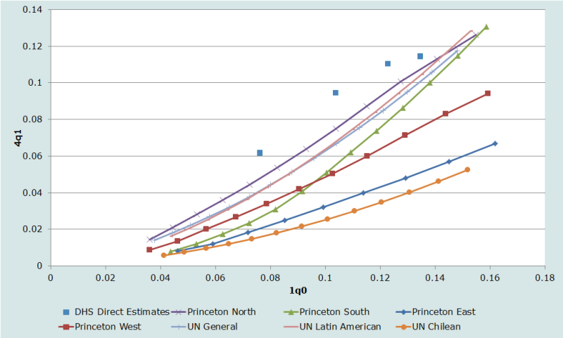
The age pattern of child mortality has an important bearing on the translation of a proportion dead into a standard nq0, and on the translation of that nq0 into a common index such as U5MR. In a population for which fairly recent FBH data exist, the model can be selected on the basis of the FBH by plotting estimates of 4q1 against those of 1q0 on a graph showing the corresponding relationships in Coale-Demeny and United Nations model life tables. If no appropriate FBH estimates exist, the selection of a model can be based on child mortality patterns in a neighbouring population. A perfect fit of the data to any model is unlikely. The analyst should select the model that best represents the range of observations available. The same model family should be used in steps 4, 5 and 6. Steps 4 and 5 have different variants, depending on whether the data being analyzed are classified by age of mother (stream a), time since first birth of mother (stream b), or duration of marriage of mother (stream c).
Data classified by age of mother (stream a)
Step 4a(1): Estimate the mean age of the age-specific fertility schedule
This sub-step is only required for analysis using one of the United Nations model life tables for developing Countries. It is calculated from age-specific fertility rates 5fx as follows:
The (x+2) term in the numerator represents the mid-point of the age group x to x+5 at the time when the births occurred. This assumes that age-specific fertility rates are calculated from information on births in the year before the survey classified by age of woman at the time of the survey (see the section on assessment of recent fertility data for more details). If age-specific rates are calculated from registered births by age of mother at the birth, the term would be (x+2.5). Note that it is only the relative pattern of fertility by age that determines the mean, so there is no need to adjust level by, for example, a relational Gompertz model, before calculating it.
Step 4a(2): Estimate nq0 from each 5PDx
Once a model life table family j has been identified, appropriate parameters a(x,j), b(x,j) and c(x,j) (and d(x,j) if a UN model life table is being used) are substituted into the following equation:
Note that d(x,j) is zero unless using the UN Model Life Tables.
Table 1: Values of a(x,j), b(x,j), c(x,j) and optional d(x,j) for estimating probabilities of dying by exact ages of childhood from proportions dead of children ever born classified by age of mother
|
|
|
Age group of mother and value of n in nq0 |
||||||
|
Family j |
Coefficient |
15-19 |
20-24 |
25-29 |
30-34 |
35-39 |
40-44 |
45-49 |
|
Value of n in nq0 |
1 |
2 |
3 |
5 |
10 |
15 |
20 |
|
|
Princeton 'North' |
a(x,j) |
1.1119 |
1.2390 |
1.1884 |
1.2046 |
1.2586 |
1.2240 |
1.1772 |
|
b(x,j) |
-2.9287 |
-0.6865 |
0.0421 |
0.3037 |
0.4236 |
0.4222 |
0.3486 |
|
|
c(x,j) |
0.8507 |
-0.2745 |
-0.5156 |
-0.5656 |
-0.5898 |
-0.5456 |
-0.4624 |
|
|
Princeton 'South' |
a(x,j) |
1.0819 |
1.2846 |
1.2223 |
1.1905 |
1.1911 |
1.1564 |
1.1307 |
|
b(x,j) |
-3.0005 |
-0.6181 |
0.0851 |
0.2631 |
0.3152 |
0.3017 |
0.2596 |
|
|
c(x,j) |
0.8689 |
-0.3024 |
-0.4704 |
-0.4487 |
-0.4291 |
-0.3958 |
-0.3538 |
|
|
Princeton 'East' |
a(x,j) |
1.1461 |
1.2231 |
1.1593 |
1.1404 |
1.1540 |
1.1336 |
1.1201 |
|
b(x,j) |
-2.2536 |
-0.4301 |
0.0581 |
0.1991 |
0.2511 |
0.2556 |
0.2362 |
|
|
c(x,j) |
0.6259 |
-0.2245 |
-0.3479 |
-0.3487 |
-0.3506 |
-0.3428 |
-0.3268 |
|
|
Princeton 'West' |
a(x,j) |
1.1415 |
1.2563 |
1.1851 |
1.1720 |
1.1865 |
1.1746 |
1.1639 |
|
b(x,j) |
-2.7070 |
-0.5381 |
0.0633 |
0.2341 |
0.3080 |
0.3314 |
0.3190 |
|
|
c(x,j) |
0.7663 |
-0.2637 |
-0.4177 |
-0.4272 |
-0.4452 |
-0.4537 |
-0.4435 |
|
|
United Nations 'Latin America' |
a(x,j) |
0.6892 |
1.3625 |
1.0877 |
0.7500 |
0.5605 |
0.5024 |
0.5326 |
|
b(x,j) |
-1.6937 |
-0.3778 |
0.0197 |
0.0532 |
0.0222 |
0.0028 |
0.0052 |
|
|
c(x,j) |
0.6464 |
-0.2892 |
-0.2986 |
-0.1106 |
0.0170 |
0.0048 |
0.0256 |
|
|
d(x,j) |
0.0106 |
-0.0041 |
0.0024 |
0.0115 |
0.0171 |
0.0180 |
0.0168 |
|
|
United Nations 'Chilean' |
a(x,j) |
0.8274 |
1.3129 |
1.0632 |
0.8236 |
0.6895 |
0.6098 |
0.5615 |
|
b(x,j) |
-1.5854 |
-0.2457 |
0.0196 |
0.0293 |
0.0068 |
-0.0014 |
0.0040 |
|
|
c(x,j) |
0.5949 |
-0.2329 |
-0.1996 |
-0.0684 |
0.0032 |
0.0166 |
0.0073 |
|
|
d(x,j) |
0.0097 |
-0.0031 |
0.0021 |
0.0081 |
0.0119 |
0.0141 |
0.0159 |
|
|
United Nations 'South Asian' |
a(x,j) |
0.6749 |
1.3716 |
1.0899 |
0.7694 |
0.6156 |
0.6077 |
0.6952 |
|
b(x,j) |
-1.7580 |
-0.3652 |
0.0299 |
0.0548 |
0.0231 |
0.0040 |
0.0018 |
|
|
c(x,j) |
0.6805 |
-0.2966 |
-0.2887 |
-0.0934 |
0.0298 |
0.0573 |
0.0306 |
|
|
d(x,j) |
0.0109 |
-0.0041 |
0.0024 |
0.0108 |
0.0149 |
0.0141 |
0.0109 |
|
|
United Nations 'Far Eastern' |
a(x,j) |
0.7194 |
1.2671 |
1.0668 |
0.7833 |
0.5765 |
0.4115 |
0.3071 |
|
b(x,j) |
-1.3143 |
-0.2996 |
0.0017 |
0.0307 |
0.0068 |
0.0014 |
0.0111 |
|
|
c(x,j) |
0.5432 |
-0.2105 |
-0.2424 |
-0.1103 |
-0.0202 |
0.0083 |
0.0129 |
|
|
d(x,j) |
0.0093 |
-0.0029 |
0.0019 |
0.0098 |
0.0165 |
0.0213 |
0.0251 |
|
|
United Nations 'General' |
a(x,j) |
0.7210 |
1.3115 |
1.0768 |
0.7682 |
0.5769 |
0.4845 |
0.4760 |
|
b(x,j) |
-1.4686 |
-0.3360 |
0.0109 |
0.0439 |
0.0176 |
0.0034 |
0.0071 |
|
|
c(x,j) |
0.5746 |
-0.2475 |
-0.2695 |
-0.1090 |
0.0038 |
0.0036 |
0.0246 |
|
|
d(x,j) |
0.0095 |
-0.0034 |
0.0021 |
0.0105 |
0.0165 |
0.0187 |
0.0189 |
|
|
Sources: Princeton models: UN Population Division (1983); UN Models: UN Population Division (1991) |
||||||||
For each age group (x,x + 5), nq0 is estimated by multiplying the right-hand side of the equation by the empirically-observed 5PDx.
Step 5a: Estimate the time reference t(x) of each estimated nq0
Using the model life table family j identified as being appropriate, parameters e(x,j), f(x,j) and g(x,j) are substituted into the following equation:
The location of the estimates in calendar time is readily achieved by subtracting the t(x) from the census or survey date (Table 2).
Table 2: Values of e(x,j), f(x,j) and g(x,j) for estimating the reference period t(x) for probabilities of dying by exact ages of childhood from proportions dead of children ever born classified by age of mother
|
|
|
Age group of mother and value of n in nqx |
||||||
|
Family j |
Coefficient |
15-19 |
20-24 |
25-29 |
30-34 |
35-39 |
40-44 |
45-49 |
|
Value of n in nq0 |
1 |
2 |
3 |
5 |
10 |
15 |
20 |
|
|
Princeton 'North' |
e(x,j) |
1.0921 |
1.3207 |
1.5996 |
2.0779 |
2.7705 |
4.1520 |
6.9650 |
|
f(x,j) |
5.4732 |
5.3751 |
2.6268 |
-1.7908 |
-7.3403 |
-12.2448 |
-13.9160 |
|
|
g(x,j) |
-1.9672 |
0.2133 |
4.3701 |
9.4126 |
14.9352 |
19.2349 |
19.9542 |
|
|
Princeton 'South' |
e(x,j) |
1.0900 |
1.3079 |
1.5173 |
1.9399 |
2.6157 |
4.0794 |
7.1796 |
|
f(x,j) |
5.4443 |
5.5568 |
2.6755 |
-2.2739 |
-8.4819 |
-13.8308 |
-15.3880 |
|
|
g(x,j) |
-1.9721 |
0.2021 |
4.7471 |
10.3876 |
16.5153 |
21.1866 |
21.7892 |
|
|
Princeton 'East' |
e(x,j) |
1.0959 |
1.2921 |
1.5021 |
1.9347 |
2.6197 |
4.1317 |
7.3657 |
|
f(x,j) |
5.5864 |
5.5897 |
2.4692 |
-2.6419 |
-8.9693 |
-14.3550 |
-15.8083 |
|
|
g(x,j) |
-1.9949 |
0.3631 |
5.0927 |
10.8533 |
17.0981 |
21.8247 |
22.3005 |
|
|
Princeton 'West' |
e(x,j) |
1.0970 |
1.3062 |
1.5305 |
1.9991 |
2.7632 |
4.3468 |
7.5242 |
|
f(x,j) |
5.5628 |
5.5677 |
2.5528 |
-2.4261 |
-8.4065 |
-13.2436 |
-14.2013 |
|
|
g(x,j) |
-1.9956 |
0.2962 |
4.8962 |
10.4282 |
16.1787 |
20.1990 |
20.0162 |
|
|
United Nations 'Latin America' |
e(x,j) |
1.1703 |
1.6955 |
1.8296 |
2.1783 |
2.8836 |
4.4580 |
6.9351 |
|
f(x,j) |
0.5129 |
4.1320 |
2.9020 |
-2.5688 |
-10.3282 |
-17.1809 |
-19.3871 |
|
|
g(x,j) |
-0.3850 |
-0.1635 |
3.4707 |
9.0883 |
15.4301 |
20.4296 |
23.4007 |
|
|
United Nations 'Chilean' |
e(x,j) |
1.3092 |
1.6897 |
1.8368 |
2.2036 |
2.9955 |
4.7734 |
7.4495 |
|
f(x,j) |
1.9474 |
4.6176 |
2.6370 |
-3.3520 |
-11.4013 |
-17.8850 |
-19.0513 |
|
|
g(x,j) |
-0.7982 |
-0.0173 |
4.0305 |
9.9233 |
16.3441 |
20.8883 |
23.0529 |
|
|
United Nations 'South Asian' |
e(x,j) |
1.1922 |
1.7173 |
1.8631 |
2.1808 |
2.7654 |
4.1378 |
6.4885 |
|
f(x,j) |
0.7940 |
4.3117 |
2.8767 |
-2.7219 |
-10.8808 |
-18.6219 |
-22.2001 |
|
|
g(x,j) |
-0.5425 |
-0.1653 |
3.5848 |
9.3705 |
16.2255 |
22.2390 |
26.4911 |
|
|
United Nations 'Far Eastern' |
e(x,j) |
1.2779 |
1.7471 |
1.9107 |
2.3172 |
3.2087 |
5.1141 |
7.6383 |
|
f(x,j) |
1.5714 |
4.2638 |
2.7285 |
-2.6259 |
-9.8891 |
-15.3263 |
-15.5739 |
|
|
g(x,j) |
-0.6994 |
-0.0752 |
3.5881 |
9.0238 |
14.7339 |
18.2507 |
19.7669 |
|
|
United Nations 'General' |
e(x,j) |
1.2136 |
1.7025 |
1.8360 |
2.1882 |
2.9682 |
4.6526 |
7.1425 |
|
f(x,j) |
0.9740 |
4.1569 |
2.8632 |
-2.6521 |
-10.3053 |
-16.6920 |
-18.3021 |
|
|
g(x,j) |
-0.5247 |
-0.1232 |
3.5220 |
9.1961 |
15.3161 |
19.8534 |
22.4168 |
|
|
Sources: Princeton models: UN Population Division (1983); UN Models: UN Population Division (1991) |
||||||||
Data classified by time since first birth of mother (stream b)
Step 4b: Estimate nq0 from each 5PDx
Once a model life table family j has been identified, appropriate parameters a(x,j), b(x,j) and c(x,j) are substituted into the following equation:
Table 3: Values of a(x,j), b(x,j), c(x,j) for estimating probabilities of dying by exact ages of childhood from proportions dead of children ever born classified by time since first birth of mother
|
|
|
Time since first birth of mother and value of n in nq0 |
||||
|
Family j |
Coefficient |
0-4 |
5-9 |
10-14 |
15-19 |
20-24 |
|
Value of n in nq0 |
2 |
5 |
5 |
5 |
10 |
|
|
Princeton 'North' |
a(x,j) |
1.1980 |
1.2248 |
1.2076 |
1.2030 |
1.3292 |
|
b(x,j) |
-0.1266 |
-0.1919 |
-0.0105 |
0.0896 |
0.1598 |
|
|
c(x,j) |
0.0038 |
-0.0870 |
-0.2911 |
-0.4265 |
-0.5778 |
|
|
Princeton 'South' |
a(x,j) |
1.1705 |
1.3166 |
1.2952 |
1.2836 |
1.5269 |
|
b(x,j) |
-0.1461 |
-0.3157 |
-0.0423 |
0.1308 |
0.2659 |
|
|
c(x,j) |
0.0051 |
-0.0971 |
-0.4295 |
-0.6496 |
-0.9174 |
|
|
Princeton 'East' |
a(x,j) |
1.2182 |
1.2769 |
1.2731 |
1.2585 |
1.3410 |
|
b(x,j) |
-0.1809 |
-0.2268 |
0.0005 |
0.1216 |
0.1749 |
|
|
c(x,j) |
0.0214 |
-0.1052 |
-0.3720 |
-0.5013 |
-0.5964 |
|
|
Princeton 'West' |
a(x,j) |
1.2049 |
1.2573 |
1.2431 |
1.2469 |
1.4258 |
|
b(x,j) |
-0.1553 |
-0.2266 |
-0.0230 |
0.0999 |
0.1948 |
|
|
c(x,j) |
0.0135 |
-0.0944 |
-0.3409 |
-0.5267 |
-0.7454 |
|
Note: the coefficients and values of n in nq0 have been updated by Hill from those published in Hill and Figueroa (2001).
For each age group (x,x + 5), nq0 is estimated by multiplying the right-hand side of the equation by the empirically-observed 5PDx (Table 3).
Step 5b: Estimate the time reference t(x) of each estimated nq0
Using the model life table family j identified as being appropriate, parameters e(x,j), f(x,j) and g(x,j) are substituted into the following equation:
Table 4: Values of e(x,j), f(x,j) and g(x,j) for estimating the reference period t(x) for probabilities of dying by exact ages of childhood from proportions dead of children ever born classified by time since first birth of mother
|
|
|
Time since first birth of mother and value of n in nq0 |
||||
|
Family j |
Coefficient |
0-4 |
5-9 |
10-14 |
15-19 |
20-24 |
|
Value of n in nq0 |
2 |
5 |
5 |
5 |
10 |
|
|
Princeton 'North' |
e(x,j) |
1.71 |
2.16 |
0.66 |
-1.96 |
-3.85 |
|
f(x,j) |
1.07 |
4.36 |
3.50 |
-0.90 |
-6.42 |
|
|
g(x,j) |
-0.35 |
0.12 |
6.65 |
17.66 |
28.94 |
|
|
Princeton 'South' |
e(x,j) |
1.68 |
2.29 |
1.19 |
-1.01 |
-2.68 |
|
f(x,j) |
0.96 |
3.84 |
3.45 |
-0.18 |
-5.06 |
|
|
g(x,j) |
-0.32 |
-0.01 |
5.41 |
15.03 |
25.21 |
|
|
Princeton 'East' |
e(x,j) |
1.68 |
2.19 |
0.71 |
-1.96 |
-4.06 |
|
f(x,j) |
0.99 |
4.28 |
3.63 |
-0.71 |
-6.35 |
|
|
g(x,j) |
-0.33 |
0.02 |
6.36 |
17.42 |
29.14 |
|
|
Princeton 'West' |
e(x,j) |
1.70 |
2.20 |
0.86 |
-1.46 |
-2.97 |
|
f(x,j) |
1.03 |
4.20 |
3.47 |
-0.69 |
-5.80 |
|
|
g(x,j) |
-0.34 |
0.06 |
6.21 |
16.49 |
26.65 |
|
Note: the coefficients and values of n in nq0 have been updated by Hill from those published in Hill and Figueroa (2001).
Data classified by duration of marriage of mother (stream c)
Step 4c: Estimate nq0 from each 5PDx
Once a model life table family j has been identified, appropriate parameters a(x,j), b(x,j) and c(x,j) are substituted into the following equation:
Table 5: Values of a(x,j), b(x,j), c(x,j) for estimating probabilities of dying by exact ages of childhood from proportions dead of children ever born classified by duration of marriage of mother
|
|
|
Duration of marriage of mother and value of n in nq0 |
|||||
|
Family j |
Coefficient |
0-4 |
5-9 |
10-14 |
15-19 |
20-24 |
25-29 |
|
Value of n in nq0 |
2 |
3 |
5 |
10 |
15 |
20 |
|
|
Princeton 'North' |
a(x,j) |
1.2615 |
1.1957 |
1.3067 |
1.4701 |
1.5039 |
1.4798 |
|
b(x,j) |
-0.5340 |
-0.4103 |
-0.0103 |
0.1763 |
0.0039 |
-0.2487 |
|
|
c(x,j) |
0.1252 |
-0.0930 |
-0.4618 |
-0.7268 |
-0.7071 |
-0.5582 |
|
|
Princeton 'South' |
a(x,j) |
1.3103 |
1.2309 |
1.2774 |
1.3493 |
1.3592 |
1.3532 |
|
b(x,j) |
-0.5856 |
-0.3463 |
0.0336 |
0.1366 |
-0.0315 |
-0.1978 |
|
|
c(x,j) |
0.1367 |
-0.1073 |
-0.3987 |
-0.5403 |
-0.4944 |
-0.4099 |
|
|
Princeton 'East' |
a(x,j) |
1.2299 |
1.1611 |
1.2036 |
1.2773 |
1.3014 |
1.3160 |
|
b(x,j) |
-0.3998 |
-0.2451 |
0.0171 |
0.1015 |
-0.0219 |
-0.1630 |
|
|
c(x,j) |
0.0910 |
-0.0797 |
-0.2992 |
-0.4276 |
-0.4195 |
-0.3751 |
|
|
Princeton 'West' |
a(x,j) |
1.2584 |
1.1841 |
1.2446 |
1.3353 |
1.3875 |
1.4227 |
|
b(x,j) |
-0.4683 |
-0.3006 |
0.0131 |
0.1157 |
-0.0193 |
-0.1954 |
|
|
c(x,j) |
0.1080 |
-0.0892 |
-0.3555 |
-0.5245 |
-0.5472 |
-0.5127 |
|
For each age group (x,x+5), nq0 is estimated by multiplying the right-hand side of the equation by the empirically-observed 5PDx.
Step 5c: Estimate the time reference t(x) of each estimated nq0
Using the model life table family j identified as being appropriate, parameters e(x,j), f(x,j) and g(x,j) are substituted into the following equation:
The results are presented in Table 6.
Table 6: Values of e(x,j), f(x,j) and g(x,j) for estimating reference period t(x) for probabilities of dying by exact ages of childhood from proportions dead of children ever born classified by duration of marriage of mother
|
|
|
Duration of marriage of mother and value of n in nq0 |
|||||
|
Family j |
Coeff-icient |
0-4 |
5-9 |
10-14 |
15-19 |
20-24 |
25-29 |
|
Value of n in nq0 |
2 |
3 |
5 |
10 |
15 |
20 |
|
|
Princeton 'North' |
e(x,j) |
1.03 |
1.70 |
1.43 |
-0.08 |
-1.97 |
-2.19 |
|
f(x,j) |
1.31 |
4.21 |
3.27 |
-1.08 |
-3.48 |
0.61 |
|
|
g(x,j) |
-0.33 |
-0.02 |
4.41 |
12.93 |
21.33 |
23.94 |
|
|
Princeton 'South' |
e(x,j) |
1.02 |
1.66 |
1.21 |
-0.65 |
-2.91 |
-3.16 |
|
f(x,j) |
1.31 |
4.51 |
3.47 |
-1.60 |
-4.14 |
1.21 |
|
|
g(x,j) |
-0.33 |
-0.03 |
4.95 |
14.68 |
24.01 |
26.35 |
|
|
Princeton 'East' |
e(x,j) |
1.04 |
1.64 |
1.11 |
-0.86 |
-3.22 |
-3.39 |
|
f(x,j) |
1.42 |
4.70 |
3.30 |
-1.97 |
-4.11 |
1.67 |
|
|
g(x,j) |
-0.35 |
0.06 |
5.45 |
15.52 |
24.86 |
26.98 |
|
|
Princeton 'West' |
e(x,j) |
1.03 |
1.67 |
1.21 |
-0.54 |
-2.47 |
-2.21 |
|
f(x,j) |
1.37 |
4.59 |
3.33 |
-1.77 |
-3.92 |
1.31 |
|
|
g(x,j) |
-0.34 |
0.02 |
5.14 |
14.64 |
23.10 |
24.45 |
|
Step 6: Convert each estimate of nq0 into an estimate of 5q0
In the applications of the indirect child mortality estimation method presented here, each of the probabilities of dying by exact ages of childhood, nq0, is converted into a value of α, the level parameter of a system of relational logit model life tables. The α is then used to estimate the corresponding probability of dying between birth and exact age 5,
5q0:
where the estimates of nq0 come from Step 4 and the Ys(n) values are logit transformations of the standard life table. Thus, one obtains a series of values of α corresponding to the probabilities of dying estimated from data on the different age groups of respondents. Then for each α:
To apply the relational model approach, it is necessary to choose a standard life table. In order to apply the indirect estimation procedure, it is necessary for Steps 4 and 5 to identify an appropriate model pattern, and the standard should be drawn from the same model family. The precise level of mortality within the family is less important than the family itself (the appropriate selection of which allows β to be assumed to be 1 in the relational logit model life table). We therefore recommend choosing a standard with a life expectancy of 60 years.
Step 7: Identify and interpret the results
The resulting estimates of nq0 for each age group, the corresponding estimates of 5q0, the time location estimates, and the time trend in 5q0 must then be assessed. Plotted against time, the series of values of 5q0 will give an indication of the time trend in levels of child mortality. If data from more than one census or survey are available, estimates of 5q0 can be compared for the same time periods to evaluate the consistency and reliability of the data.
Worked example
The example uses data on children ever born and children surviving by age of mother from the 2008 Census of Malawi. The method is implemented in the associated Excel workbook.
Step 1: Calculate proportions dead of children ever born, 5PDx
Table 7 shows the basic data on number of women, number of children ever born, and number of children surviving by five-year age group of mother from the 2008 Malawi Census. The proportion dead of children ever born 5PDx is calculated by dividing the number of surviving children by the number of children ever born, and subtracting the result from 1:
The results are shown in the fifth and sixth columns of Table 7.
Table 7: Children ever born and children surviving, Malawi, 2008 Census
|
Age group x,x+4 |
Number of women |
Children ever born |
Children surviving |
Mean children ever born |
Mean children surviving |
Proportion dead, 5PDx |
|
15-19 |
635,927 |
180,178 |
161,541 |
0.2833 |
0.2540 |
0.1034 |
|
20-24 |
678,071 |
1,038,556 |
919,584 |
1.5316 |
1.3562 |
0.1145 |
|
25-29 |
566,350 |
1,613,374 |
1,398,776 |
2.8487 |
2.4698 |
0.1330 |
|
30-34 |
405,602 |
1,697,566 |
1,426,516 |
4.1853 |
3.5170 |
0.1597 |
|
35-39 |
298,004 |
1,553,676 |
1,266,514 |
5.2136 |
4.2500 |
0.1848 |
|
40-44 |
221,274 |
1,335,242 |
1,043,357 |
6.0343 |
4.7152 |
0.2186 |
|
45-49 |
174,875 |
1,128,423 |
851,048 |
6.4527 |
4.8666 |
0.2458 |
Step 2: Calculate average numbers of children ever born to women in each five-year group, 5Px
Although the average number of children born to women in each five-year age group, 5Px, is only needed for the age groups 15-19, 20-24 and 25-29, it is recommended to calculate these values for all age groups as part of data evaluation. The average is calculated simply by dividing children ever born by the number of women in the age group:
The results are shown in the sixth column of Table 7. The required parity ratios are then calculated as follows:
and
Step 3: Select a model life table family
A single set of proportions dead by age of mother contains essentially no information about the age pattern of child mortality in a population. However, in an actual country analysis, there would invariably be some other relevant information to guide a choice. The ideal information is the age pattern of child mortality from a full birth history for the same population. The comparison is of 1q0 and 4q1, and it is generally made graphically, superimposing observed points over curves showing the relationship at different mortality levels in each model family.
Several full birth history surveys have been conducted in Malawi. Figure 1 plots direct estimates for the 0 to 4 years before the DHS surveys of 1992, 2000 and 2004 (and also the 5 to 9 years before the 2000 survey) against model patterns. (Note that only three of the United Nations patterns are shown. This is because the General, South Asian, and Far Eastern patterns are indistinguishable in their age pattern of mortality under age 5.) All the observations show higher 4q1 relative to 1q0 than any of the model patterns. The optimal model choice in this instance would probably be the Princeton ‘North’ family, and it is this model that we use in what follows.
Step 4a(1): Estimate the mean age of the age-specific fertility schedule
We are using the Princeton 'North' family of model life tables, but for illustrative purposes, we estimate the mean age of the fertility schedule. The Malawi 2008 Census included a question for women of reproductive age on how many births they had in the year before the census. Table 8 shows the basic data, and the calculation of .
Table 8: Calculation of mean age of childbearing
|
Age group x,x+4 |
Number of women |
Births in previous 12 months |
Age-specific fertility rates, 5fx |
Mid-point of age group (x+2) |
5fx.(x+2) |
|
15-19 |
635,927 |
70,737 |
0.1112 |
17 |
1.891 |
|
20-24 |
678,071 |
169,406 |
0.2498 |
22 |
5.496 |
|
25-29 |
566,350 |
130,331 |
0.2301 |
27 |
6.213 |
|
30-34 |
405,602 |
79,232 |
0.1953 |
32 |
6.251 |
|
35-39 |
298,004 |
43,747 |
0.1468 |
37 |
5.432 |
|
40-44 |
221,274 |
13,956 |
0.0721 |
42 |
3.029 |
|
45-49 |
174,875 |
5,599 |
0.0320 |
47 |
1.505 |
|
Sum |
|
1.0375 |
29.817 |
is then calculated as the sum of column (vi) divided by the sum of column (iv), = 29.817/1.0375 = 28.74.
Step 4a(2): Estimate nq0 from each 5PDx
Each 5PDx is then converted into an estimated nq0 using the appropriate coefficients from Table 3, as shown in Table 9. Thus for the age group 30-34,
.
Table 9: Estimation of nq0 from each 5PDx
|
Age Group |
Proportion dead of CEB |
Regression coefficients for nq0 (Princeton 'North' Model) |
nq0 |
||
|
a(i) |
b(i) |
c(i) |
|||
|
15-19 |
0.1034 |
1.1119 |
-2.9287 |
0.8507 |
0.1063 |
|
20-24 |
0.1146 |
1.2390 |
-0.6865 |
-0.2745 |
0.1105 |
|
25-29 |
0.1330 |
1.1884 |
0.0421 |
-0.5156 |
0.1222 |
|
30-34 |
0.1597 |
1.2046 |
0.3037 |
-0.5656 |
0.1528 |
|
35-39 |
0.1848 |
1.2586 |
0.4236 |
-0.5898 |
0.1885 |
|
40-44 |
0.2186 |
1.2240 |
0.4222 |
-0.5456 |
0.2205 |
|
45-49 |
0.2458 |
1.1772 |
0.3486 |
-0.4624 |
0.2441 |
Step 5: Estimate the time reference t(x) of each estimated nq0
The time reference t(x) of each estimate before the survey or census is then obtained, using the appropriate coefficients from Table 4, as shown in Table 10. Thus for the age group 30-34,
.
The Census was taken between 8 and 28 June 2008, so the estimated reference date can be found by subtracting t from 2008.46 (the decimal year representation of 18 June 2008). Results are shown in the last column of Table 10.
Table 10: Estimation of time reference t(x) of each estimate in years before the census, Malawi, 2008 Census
|
Regression coefficients for time ago Princeton 'North' model |
Time ago t |
Reference date |
|||
|
Age group |
e(i) |
f(i) |
g(i) |
(2008.46-t) |
|
|
15-19 |
1.0921 |
5.4732 |
-1.9672 |
1.05 |
2007.42 |
|
20-24 |
1.3207 |
5.3751 |
0.2123 |
2.43 |
2006.03 |
|
25-29 |
1.5996 |
2.6268 |
4.3701 |
4.44 |
2004.03 |
|
30-34 |
2.0779 |
-1.7908 |
9.4126 |
6.81 |
2001.66 |
|
35-39 |
2.7705 |
-7.3403 |
14.9352 |
9.44 |
1999.02 |
|
40-44 |
4.1520 |
-12.2448 |
19.2349 |
12.23 |
1996.24 |
|
45-49 |
6.9650 |
-13.9160 |
19.9542 |
15.12 |
1993.35 |
Step 6: Convert each estimate of nq0 into an estimate of 5q0
The final step is to convert each estimated nq0 into an estimate of the common index . This will make it possible to compare estimates across age groups. Each nq0 is converted into its logit Y(n) by means of the identity Y(n)=0.5.ln(nq0/(1-nq0)). The value of α is then found by subtracting the standard logit Ys(n), from the North joint-sex model life tables with an expectation of life at birth of 60 years (column (vi)) from Y(n). Each α is then used with the standard Ys(5) to get the estimated . Thus for the age group 25-29, Y(3) = 0.5.ln(0.1222/(1-0.1222)) = -0.9857, and α = -0.9857 - (-1.1664) = 0.1806. Then,
Estimates of are derived in analogous fashion using the standard logit for age 1.
Table 11: Estimating the logit life table parameter α for each estimate, and deriving a set of and
|
Age group |
nq0 |
n |
logit Y(n) |
Standard logit Ys(n) |
α |
||
|
15-19 |
0.1063 |
1 |
-1.0647 |
-1.3300 |
0.2653 |
0.1063 |
0.1612 |
|
20-24 |
0.1105 |
2 |
-1.0431 |
-1.2273 |
0.1842 |
0.0918 |
0.1405 |
|
25-29 |
0.1222 |
3 |
-0.9857 |
-1.1664 |
0.1806 |
0.0912 |
0.1396 |
|
30-34 |
0.1528 |
5 |
-0.8566 |
-1.0900 |
0.2334 |
0.1004 |
0.1528 |
|
35-39 |
0.1885 |
10 |
-0.7299 |
-1.0091 |
0.2791 |
0.1089 |
0.1650 |
|
40-44 |
0.2205 |
15 |
-0.6313 |
-0.9664 |
0.3350 |
0.1203 |
0.1809 |
|
45-49 |
0.2441 |
20 |
-0.5652 |
-0.9138 |
0.3487 |
0.1232 |
0.1850 |
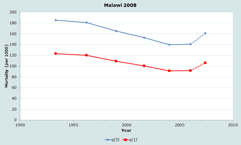
Figure 2 plots each estimate of and against the corresponding reference date. The figure indicates a declining trend in under-five mortality over time, from around per 1000 in the early 1990s to around 140 in 2005. The apparent uptick in child mortality in 2007 is to be disregarded owing to the likely exaggeration of mortality estimated from very young mothers, as discussed above.
Diagnostics, analysis and interpretation
Checks and validation
Regardless of how data have been collected, or of one’s knowledge of how thoroughly interviewers were trained and supervised, careful data quality review is an essential first step of any analysis. All data sets contain errors, which can result from many sources, such as an interviewer cutting corners or an interviewee simply not knowing the correct answer to a question.
One specific aspect of summary birth history data needs to be emphasized for the data checking, and that is the failure of assumption 2, that mortality risks of children for a particular time period do not vary by age of mother. In many applications it is abundantly clear that this assumption does not hold. The risks for children of women aged 15-19 (and the indirect estimate of child mortality based on CEB and CD for this age group) are frequently higher, sometimes very substantially so, than the population average. The same is true to a lesser extent for the children of mothers aged 20-24. Two factors account for this distortion: the distribution of children by birth order and socio-economic factors. First births are known to be at higher risk of dying than higher-order births, and the children born to younger women clearly consist of an above-average proportion of first births. Women having children at early ages also tend to come from below-average socio-economic groups, and their children are thus exposed to above-average mortality risks. Consequently the estimates of mortality derived from women aged 15-19 should be treated with a high degree of circumspection, or ignored altogether.
Interpretation
Two key characteristics of this method need to be borne in mind when interpreting results. First, there is no information about specific dates or ages in the basic data. The only timing information in the number of children ever borne by a woman is that those births occurred at some point between when she had her first birth and her age at the time of the survey. Even less information is available from the number of those children that have died about ages at death, since possible age ranges depend on time distributions of births. It is thus impossible to draw conclusions about short-term fluctuations in child mortality from a SBH. Reports of two women of the same age (duration of marriage, time since first birth) reporting the same numbers of children ever born and died can reflect experiences of different mortality conditions. The best that a summary birth history can offer is a broad indication of an average past trend. Even this average trend needs to be interpreted with care for the recent past because of the selection biases affecting reports of women aged 15-19 and, though to a lesser extent, 20-24.
The second characteristic is that information is provided only for surviving women who still live in surveyed households, with an associated risk of respondent selection bias. The mortality experience of children born in a community whose mothers no longer live in the community will not be included in the measures. If such children have higher mortality than those born to mothers who do still live in the community, mortality will be under-estimated. The most severe form of this bias is likely to result from substantial levels of HIV prevalence in the community, since such prevalence in the absence of widespread antiretroviral therapy will result in a strong positive correlation between survival of child and survival of mother (described in the section on the effects of HIV on methods for child mortality estimation). However, some positive correlation between mother and child survival is almost certain in any population.
There are also other possible sources of respondent selection bias. For example, high in-migration rates will result in women reporting on the survival of children born and raised elsewhere, while high out-migration will remove responses about children who were born and raised in the community. Though it is impossible to know a priori the direction or magnitude of such biases, the analyst needs to keep in mind their potential effect. Non-response itself may actually be a smaller problem for the summary birth history than the full birth history, since information is often collected from third parties, not necessarily from the woman herself. Thus a summary birth history for a woman absent from the community on an extended trip might be collected when a full birth history for the same woman would not be since she could not be interviewed in person.
Detailed description of method
The idea that proportions of children dead among children ever born were indicators of child mortality has a long history. Questions on children ever born and children surviving were included in the 1900 Census of the United States (Preston and Haines 1991), the 1911 Census of Britain, and the 1940 Census of Brazil, among others. However, the first methodology for translating such proportions into standard life table indicators was proposed by Brass and Coale (1968).
To illustrate the basic idea, take a simple if implausible example of a population in which all women have exactly one child, born at exact age 25, that all the women survive from age 25 to age 30, and that there is no migration. In a survey, the proportion dead among children borne by women of exact age 30 will precisely measure the cohort probability of dying between birth and exact age 5, 5q0. In another population, all women also have exactly one child, but at age 27; in this population, the proportion dead will precisely measure the cohort probability of dying by age 3, 3q0.
These two examples illustrate a number of important points. First, age of the women is a proxy for the exposure to risk of their children. Other things being equal, the older the mother, the longer on average her children have been exposed to the risk of dying. Second, the interpretation of a proportion dead of children ever born in terms of a standard life table measure depends on the age of childbearing. Third, equivalence of a proportion dead to a life table measure requires that there be no selection effects by mortality or out migration, nor contamination effects by in-migration. Fourth, the measures obtained are for cohorts (or averages across cohorts) rather than for time periods.
Of course in real populations children are born at a range of ages of mother and are exposed to age-specific mortality risks that may change over time. Estimation methods use model age patterns of fertility and child mortality to create model proportions dead of children ever born that can then be related to underlying life table parameters. A common feature of data on survival of children classified by age group of mother is that proportions dead for women aged 15-19 and 20-24 are higher than for subsequent age groups, despite the fact that they reflect shorter average exposure times of children. The problem arises because young women who have children are generally of below average socio-economic status, and their children are disproportionately first births, both of which are known risk factors for high child mortality. The experience of the children of such young mothers is therefore not representative of all children born in the population. Partly to address this bias, methods have been developed classifying women by duration of marriage (Sullivan 1972) and time since first birth (Hill and Figueroa 2001). It is also argued that these methods are less affected by fertility change.
The method was originally developed by Brass without explicit consideration of the effects on the estimates of mortality change, though he notes that under conditions of change “the estimates of q(2) and q(3) would be representative of the average mortality for a short period (less than a decade) before the census or survey” (Brass and Coale, 1968: 116). It is clear today that child mortality has been declining globally, and very rapidly in some populations. Following pioneering work by Feeney (1976, 1980), methods were developed to estimate a 'time reference' for the estimate derived from each age/duration group (Coale and Trussell (1977); Palloni and Heligman (1985); Hill and Figueroa (2001)). The proportion dead of CEB for a group of women represents an average of mortality risks across all the birth cohorts of their children. The older the women, or the longer their exposure, the further back in time the cohorts stretch, and the further back the reference time for a child mortality estimate based on the proportion dead. Since child mortality risks are highly concentrated at young ages, the reference date is not in practice very different from the average number of years ago that the births occurred if mortality trends have been fairly stable over time. The exact calendar year reference dates for the child mortality estimates thus have to be treated as central points in time with a distribution of deaths around them. As a result, the child mortality estimates derived from SBHs and variants of the Brass indirect methods cannot be used to identify mortality changes or crises located at a particular point in time. The method provides a good description of general trends in child mortality but smoothed in comparison with the true year-to-year fluctuations seen in almost every population. Other methods of measurement (such as FBH) are thus needed to estimate the temporal impact of, for example, health interventions on child survival.
Mathematical exposition (Manual X and UN Model Life Table methods)
The proportion dead of children ever borne by women of exact age x, PD(x), is a birth-weighted average of cohort probabilities of dying:
where f(y) is the fertility rate at age y, x-yqc0 is the probability of dying by age (x-y) for the cohort born (x-y) years earlier, and α is the earliest age of childbearing. The expression is exactly the same for duration of marriage and time since first birth, except that α becomes 0. Proportions dead for five-year age or duration groups can then be estimated by averaging point PD estimates across the group, weighting for assumed population distributions Nx at each x. It is typically assumed that the underlying population can be regarded as stable, with a growth rate appropriate for the demographic parameters underlying the PD(x), and that the underlying life table at adult ages is that used in the calculation of the PD(x). Such calculations use discrete age groups, for example, using single years of age:
Model schedules of f, q and N are used to model the 5PDx values, which are then related to appropriate q values by regression analysis using parity ratios as the independent variables (see estimating equations above).
Extensions of the method
Variants by duration of marriage or time since first birth
As described above, though not illustrated in detail, variants of the original method have been developed, classifying women by duration of marriage (Sullivan 1972) or time since first birth (Hill and Figueroa 2001). The methods were developed to address two potential sources of error in the age-based method: effects of changing fertility (primarily through distorting the parity ratios) and the above-average mortality risks of children born to young mothers.
While these variants are illustrated below, the two refinements suffer from limitations of their own. First, many population censuses do not routinely collect the information needed to tabulate women and their children by duration of marriage or time since first birth. Second, with regard to the duration of marriage approach, in many developing countries marriage is not a prerequisite for commencement of childbearing. Further, the mortality of children of unmarried mothers may well be higher than that of mothers who are married. Thus distortions may also arise in the results of these variants. Where such data are collected, as in many Arab countries with low proportions of births outside marriage, they can provide important insights into the relative performance of the different approaches.
Some surveys, for instance the MICS (Multiple Indicator Cluster Surveys, conducted under the auspices of UNICEF) carried out before about 2010, have collected summary birth histories and the necessary information on date of marriage and first birth. The question thus arises as to which variant of the methodology should be preferred.
To explore this question, we have used a full birth history survey, the 1999-2000 Bangladesh Demographic and Health Survey. The data have been tabulated in all three formats, and analysed using the Princeton ‘South’ family of model life tables. Figure 3 shows the estimates of 5q0 derived from each approach. (It may be noted that this particular data set does not show a strong over-estimation of mortality based on the most recent (15-19) age group.)
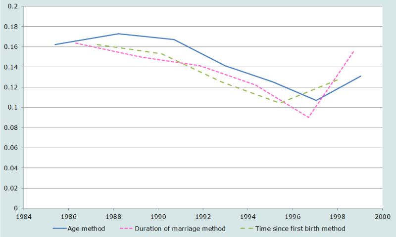
If one ignores in each series the most recent point (15-19 for age, 0-4 for both duration of marriage and time since first birth) the general trends of the estimates are very similar. The marital duration and time since first birth methods show similar levels, but from age group 25-29 onwards, the age estimates are always highest, averaging 20 per 1,000 higher (155 per 1,000) than either of the other two methods. Straight averages of all the duration of marriage and time since first birth estimates for all points except the most recent give almost the same result, 133 for marriage duration and 136 from time since first birth, although the estimates span slightly different periods.
There are several points of interest in this application. First, the marriage duration and time since first birth methods were developed in part to try to circumvent the problem of selection bias in the age-based points for women aged 15-19 and 20-24. In this application, however, these two methods show jumps for the most recent point as large as or larger than that for the age-based estimates. This could be the case if the dominant selection bias is for first births, all (time since first birth) or almost all (marriage duration) of which will be concentrated in the first category, whereas they will be more spread out across age groups.
A second issue is the use of parity ratios as observed at the time of the survey to reflect the time distribution of births in the past. As noted above, if fertility is declining (even if the relative age pattern of fertility is not changing), the parities for the younger women will be lower and those for the older women higher, reducing the parity ratios below the values for any true cohort. This will give the appearance of more recent childbearing (and thus lower average duration of child exposure to the risk of dying) than is really the case, and thus lead to over-estimates of child mortality.
Bangladesh experienced a substantial fertility decline from the mid-1980s to the time of the 1999-2000 DHS, so it is interesting to explore the size of this possible bias. Since the data come from a full birth history, we can calculate cohort parities at points 5, 10, 15 etc. years in the past by subtracting recent births from children ever born, and then calculate parity ratios for true cohorts. We can only use the standard methodology (using ratios P(1)/P(2) and P(2)/P(3)) for cohorts that have reached the third age or duration group, thus age groups 25-29 and up or time since first birth/marriage duration categories of 10-14 and up.
The first panel of Table 12 compares parity ratios at the time of survey and cohort parity ratios. The expected pattern is quite clear for the age method, with the time of survey ratios being clearly below any of the cohort ratios, which are themselves rather stable across cohorts. The picture is less clear for the marital duration and time since first birth methods however: the P(2)/P(3) ratios are generally larger than the time of survey ratios, whereas the P(1)/P(2) ratios are uniformly lower.
Table 12: Parity ratios P(1)/P(2) and P(2)/P(3) calculated at the time of survey versus for true cohorts, Bangladesh 1999-2000 DHS
|
Age method |
||||||
|
Parity ratio |
Time of survey |
Cohort aged 25-29 |
Cohort aged 30-34 |
Cohort aged 35-39 |
Cohort aged 40-44 |
Cohort aged 45-49 |
|
P(1)/P(2) |
0.269 |
0.342 |
0.311 |
0.327 |
0.361 |
0.336 |
|
P(2)/P(3) |
0.544 |
0.660 |
0.639 |
0.603 |
0.632 |
0.619 |
|
Duration of marriage method |
||||||
|
Parity ratio |
Time of survey |
Cohort 10-14 |
Cohort 15-19 |
Cohort 20-24 |
Cohort 25-29 |
|
|
P(1)/P(2) |
0.353 |
0.352 |
0.288 |
0.274 |
0.287 |
|
|
P(2)/P(3) |
0.635 |
0.682 |
0.650 |
0.598 |
0.603 |
|
|
Time since first birth method |
||||||
|
Parity ratio |
Time of survey |
Cohort 10-14 |
Cohort 15-19 |
Cohort 20-24 |
|
|
|
P(1)/P(2) |
0.553 |
0.544 |
0.495 |
0.505 |
|
|
|
P(2)/P(3) |
0.709 |
0.775 |
0.753 |
0.723 |
|
|
To get a sense of the magnitude of this effect on the estimates, we can use cohort parity ratios for each proportion dead of children ever born (for age groups 25-29 and over, and duration groups 10-14 and over). The three panels of Figure 4 show the original and cohort-based estimates by reference date, for age groups, marital duration groups and time since first birth groups respectively. The use of cohort ratios reduces the estimates based on age groups 25-29 and 30-34, but has little effect on the estimates from the other two methods. One possible explanation would be that the fertility decline in Bangladesh over this period was primarily an increase in age at childbearing, with small effects by duration of marriage or time since first birth. The net effect of using cohort ratios is to improve consistency across methods, but at the rather high cost of losing the most recent estimates.
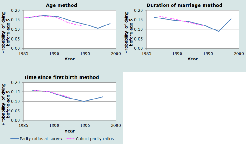
The bottom line is that the age-based method will tend to over-estimate child mortality if fertility is changing rapidly, whereas the effects on the other two approaches appear to be small. If the data are available, it is advisable to use one of the other two variants rather than the age-based method, but it may not be worth including an extra question in a census just to get this information.
Further reading and references
The indirect estimation of child mortality is discussed in all the classic manuals on indirect estimation (Sloggett, Brass, Eldridge et al. 1994; UN Population Division 1983).
Brass W and AJ Coale. 1968. "Methods of analysis and estimation," in Brass, W, AJ Coale, P Demeny, DF Heisel, et al. (eds). The Demography of Tropical Africa. Princeton NJ: Princeton University Press, pp. 88-139.
Brass W, AJ Coale, P Demeny, DF Heisel et al. (eds). 1968. The Demography of Tropical Africa. Princeton NJ: Princeton University Press.
Coale AJ and J Trussell. 1977. "Estimating the time to which Brass estimates apply; Annex I to Preston SH and Palloni A "Fine-tuning Brass-type mortality estimates with data on ages of surviving children"", Population Bulletin of the United Nations 10:87-89. https://www.un.org/development/desa/pd/content/population-bulletin-united-nations-special-issue-nos-10
Collumbien M and A Sloggett. 2001. "Adjustment methods for bias in the indirect childhood mortality estimates," in Zaba, B and J Blacker (eds). Brass Tacks: Essays in Medical Demography. London: Athlone, pp. 20-42.
Feeney G. 1976. "Estimating infant mortality rates from child survivorship data by age of mother", Asian and Pacific Census Newsletter 3(2):12-16. https://hdl.handle.net/10125/3556.
Feeney G. 1980. "Estimating infant mortality trends from child survivorship data", Population Studies 34(1):109-128. doi: https://dx.doi.org/10.1080/00324728.1980.10412839
Hill K and M-E Figueroa. 2001. "Child mortality estimation by time since first birth," in Zaba, B and J Blacker (eds). Brass Tacks: Essays in Medical Demography. London: Athlone, pp. 9-19.
Palloni A and L Heligman. 1985. "Re-estimation of structural parameters to obtain estimates of mortality in developing countries", Population Bulletin of the United Nations 18:10-33. https://www.un.org/development/desa/pd/content/population-bulletin-united-nations-special-issue-nos-18
Preston SH and MR Haines. 1991. Fatal Years: Child Mortality in Late Nineteenth-century America. Princeton, NJ: Princeton University Press.
Sloggett A, W Brass, SM Eldridge, IM Timæus, P Ward and B Zaba. 1994. Estimation of Demographic Parameters from Census Data. Tokyo, Japan: United Nations Statistical Institute for Asia and the Pacific.
Sullivan JM. 1972. "Models for the estimation of the probability of dying between birth and exact ages of early childhood", Population Studies 26(1):79-97. doi: https://dx.doi.org/10.1080/00324728.1972.10405204
UN Population Division. 1983. Manual X: Indirect Techniques for Demographic Estimation. New York: United Nations, Department of Economic and Social Affairs, ST/ESA/SER.A/81. https://www.un.org/development/desa/pd/sites/www.un.org.development.desa.pd/files/files/documents/2020/Jan/un_1983_manual_x_-_indirect_techniques_for_demographic_estimation.pdf
UN Population Division. 1991. Child Mortality in Developing Countries. New York: United Nations, Department of Economic and Social Affairs, ST/ESA/SER.A/123. https://www.un.org/development/desa/pd/content/child-mortality-developing-countries-socio-economic-differentials-trends-and-implications
- Printer-friendly version
- Log in to post comments