The relational Gompertz model
Description of method
The relational Gompertz method is a refinement of the Brass P/F ratio method that seeks to estimate age-specific and total fertility by determining the shape of the fertility schedule from data on recent births reported in censuses or surveys while determining its level from the reported average parities of younger women.
In producing estimates of age-specific and total fertility, the method seeks to remedy the errors commonly found in fertility data associated with too few or too many births being reported in the reference period, and the under-reporting of lifetime fertility and errors of age reporting among older women. These errors are described in greater detail in the section on evaluation of fertility data.
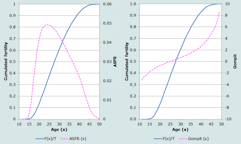
The method relies on a useful property of a (cumulated) Gompertz distribution,
which is sigmoidal (i.e. S-shaped), but also has an associated hazard function that is right-skewed and which therefore captures fairly well both the pattern of average parities of women by age and their cumulated fertility. The form of G(x) implies that a double-negative log transform of proportional cumulated fertilities or average parities approximates a straight line for most of the age range. The double-log transform,
is termed a gompit and has a close analogue in the logit transform frequently used in mortality analysis. Brass, however, found that a much closer linear fit could be obtained by a relational model that expresses the gompits of an observed series of fertility data as a linear function of the gompits of a defined standard fertility schedule. In other words,
where is the gompit of the standard fertility schedule. Evidently, if α = 0 and β = 1, the fertility schedule will be identical to the standard fertility schedule. Alpha (α) represents the extent to which the age location of childbearing in the population differs from that of the standard (negative values imply an older distribution of ages at childbearing than in the standard), while beta (β) is a measure the spread of the fertility distribution (values greater than 1 imply a narrower distribution).
As input data, the method requires average parities at each age group, for x= 15, 20, … , 45, and fertility rates in each age group, .
For ease of exposition, and to differentiate more clearly between lifetime and recent fertility data, is indexed as P(1), as P(2) and so on. The derivation of these inputs from census data is described in the section of the manual dealing with the assessment and evaluation of data on fertility. As with other methods, the average parities should be adjusted for an el-Badry correction where appropriate.
Cumulated (period) fertility to the end-point of each age group, is given by
The original method proposed by Brass (1978) used the series of the gompits of the ratio of cumulated fertility to the end of each age group to the fertility rate cumulated to age 50 (i.e. total fertility, TF), giving a sigmoidal curve with minimum of 0 and a maximum (at the last age group) of 1. Gompits of the average parities are derived in a similar manner.
There are two inherent weaknesses in this approach. First, it requires total fertility as an input, and estimates of total fertility available from reported age-specific fertility rates (ASFRs) may be biased. In fact, total fertility is often the parameter of greatest interest that the analyst is trying to estimate. The second weakness is the implicit assumption of constant fertility over time arising from the treatment of the parity gompits. Nonetheless, Brass’ formulation inspired the derivation of the standard fertility schedule by Booth (1980, 1984), which is still used in the model to this day.
Both limitations are addressed comprehensively by Zaba’s (1981) reformulation of the method, which avoids the circularity of the original method while also dropping the need to assume that fertility has been constant. Further unpublished work by Zaba generalized the approach to incorporate alternative variants of the model (some of which are described here). A full exposition of Zaba’s reformulation is given in a subsequent section. In summary, however, she showed that the model can be expressed as
(Equation 1)
where e(x), g(x) and c are functions of the chosen standard and z(x) is the gompit of the ratios of adjacent cumulated period fertility measures, i.e. F(x)/F(x+5), instead of F(x)/50 as Brass originally suggested.
In other words,
For the parity data, the model is fitted to the ratios of adjacent average parities, P(i)/P(i+1). This means that the model can be used without the need to estimate total fertility before fitting the shape parameters. It follows further from Equation 1 that a plot of z(x) - e(x) against g(x) should be a straight line with slope β and intercept
(Noting that β should be close to one, early formulations of the procedure deemed the last term of the intercept unimportant, leaving the intercept approximated by alpha. With the computing power now to hand, there is no justification for the associated loss of precision in the calculation of the intercept. However, the requirement that β be close to 1 remains).
Exactly the same reasoning holds for the evaluation of the parity data. Using P(i)/P(i+1), the ratio of average parities in successive age groups, with a linear equation relating z(i) - e(i) to g(i) results in
(Equation 2)
By convention, the points derived from the parity data are known as P-points and those derived from the fertility rates are known as F-points. The goal of the model-fitting procedure is to find a combination of P- and F-points that are internally consistent with each other (i.e. the two sets of points define essentially the same lines) and then to use these to determine jointly the parameters α and β in Equations 1 and 2 above. The values of α and β are used to derive the relational gompits, , and similarly for Y(i).
Deriving a fitted fertility distribution using the relational Gompertz method requires tabulations of calculated average parities and fertility rates by age. The fertility rates are cumulated and ratios of successive cumulated values are computed. Ratios of successive average parities are also calculated. Gompits of these ratios are calculated and used to plot the two pairs of points, z(x) - e(x) against g(x), and z(i) - e(i) against g(i). The fitted lines will have slopes equal to β, and an intercept term involving α, β and c, from which α can be calculated. The values of α and β are used to transform the gompits of the standard cumulants into fitted gompits, which are then converted to fitted average parities and fertility rates. The level of fertility is set by the most reliable parity points. These are usually those on women aged 20-29 or 20-34 who are both less likely to omit births and likely to report their ages more accurately than older women.
The use of the relational Gompertz model in the calculation of a fitted fertility distribution has a number of advantages over the earlier P/F ratio method. The model uses a reliable fertility pattern for medium- to high-fertility regimes (the Booth standard). Thus unreliable fertility rates estimated from reports of births in the last year can be replaced by model values which are fitted using the more reliable points. The plot of the two series of points is a powerful guide to the reliability of each point, and can provide insight into data errors as well as identify fertility trends. All reliable points can be used to derive the fitted model distribution. The model also provides a reliable way of interpolating between values to make parity and cumulated fertility data comparable and to convert fertility rates in unconventional age groups to rates that apply to conventional age groups.
Data requirements and assumptions
Tabulations of data required
- Fertility rates for the 12, 24 or 36 months before the survey, classified by age of mother at survey, or by age at birth of child; or
- number of women at the census or survey date, by five-year age group; and
- number of births to women in the 12, 24 or 36 months before the survey, by five-year age group.
- Average parities of women, classified by five-year age group of mother; or
- number of women, by five-year age group; and
- total number of children born to women, by five-year age group.
Important assumptions
- The standard fertility schedule chosen for use in the fitting procedure appropriately reflects the shape of the fertility distribution in the population.
- Any changes in fertility have been smooth and gradual and have affected all age groups in a broadly similar way.
- Errors in the pre-adjustment fertility rates are proportionately the same among women in the central age groups (20-39), so that the age pattern of fertility described by reported recent births is reasonably accurate.
- The parities reported by younger women (aged 20-29 or 20-34) are accurate.
The method usually allows violations of these assumptions to be detected.
Preparatory work and preliminary investigations
Before commencing analysis of fertility levels using this method, analysts should investigate the quality of the data at least in respect of the following dimensions:
- age and sex structure of the population;
- reported births in the last year; and
- average parities and the necessity of an el-Badry correction.
Caveats and warnings
- In applying this method, analysts must take particular care to ascertain and correctly specify the definition used to classify age of mother.
- Where appropriate and necessary, the average parities should be the corrected average parities after application of the el-Badry correction for the misreporting of childless women as parity not stated.
- The method can handle data aggregated over a three-year period. However, caution should be exercised in using the full model (as opposed to using it simply for smoothing) with data for periods of much longer than a year. Ideally, person-years exposed to risk should be calculated more accurately if using a longer period of investigation. In addition, there is the risk of multiple births occurring within an extended period of investigation, and the form of the questions in the census or survey instrument may be inadequate to the task of identifying such cases.
- If sample or design weights have been provided with the data, they must be applied in the manner appropriate to your statistical software when deriving the tabulations used as inputs.
- The method is contra-indicated where the shape of the fertility distribution being modelled differs markedly from that of the underlying fertility standard. Since the modelled parameters α and β define the shape and location of the fertility schedule, Zaba (1981) recommends that the model only be applied where -0.3 < α < 0.3 and 0.8 < β < 1.25. An alternative standard should be considered if α and β lie outside these ranges.
- Some of the approximations used in obtaining the estimating equations work less well for the youngest and oldest age groups than for those in the middle age range, especially if the reported fertility schedule is radically different from the standard. The points derived from the reports of these women should therefore be treated with extra caution. However, this has little impact on the estimates of Total Fertility.
Application of method
The method is applied in the following stages.
Step 1: Calculate the reported average parities
Calculate the average parities, of women in each age group [x,x+5), for x =15, 20…45, if not already done as part of the preliminary investigations, or produced as a consequence of applying the el-Badry correction. The derivation and correction of average parities is described in the section on evaluation and assessment of parity data.
Step 2: Determine the classification of the age of mother
Depending on the data available, the fertility rates may be classified either by age of mother at the survey date, or by age of mother at birth of her child. The former ages are almost always encountered in the analysis of census data, where the mother’s age is her age at the census. The latter are more commonly encountered with administrative data derived from vital registration systems. It is crucial that this classification is determined correctly as mis-specification here will bias the estimated rates produced.
The spreadsheet implementation of the model can accommodate data with no shift (i.e. reported according to the age of mother at birth); or – in the case of data classified by age of mother at survey date – with half a year, a year or one and a half year’s shift (for periods of investigation of 12, 24 and 36 months, respectively).
Step 3: Calculate implied age-specific fertility rates and parities
Age-specific fertility rates are derived by dividing the births reported in the period of investigation (e.g. the year, two years or three years) before the survey date by the number of women in each age group.
Step 4: Choose the fertility standard to be applied and the model variant to be fitted
The default fertility standard is that produced by Booth, modified slightly by Zaba (1981). The standard is appropriate to high- and medium-fertility populations and is a normalized cumulated fertility schedule (i.e. with total fertility equal to one). The standard Ys(x) values are determined by taking the gompits of the schedule and the standard parity values, Ys(i), are the gompits of the parities associated with the standard fertility schedule. The choice of standard determines the values of g() and e() used in the regression fitting procedures which are derived algebraically from the Ys().
Two variants of the relational Gompertz model are presented here. The default option is to make the same assumptions about the nature of errors inherent in fertility data as in the Brass P/F method, namely that reports of recent fertility suffer from reference-period errors and under-reporting that are independent of age, and that reports of lifetime fertility suffer from omission errors that increase with age. In the spreadsheet, this is referred to as the 'Shape F – Level P' variant.
A second variant involves using the relational Gompertz model to correct for possible distortions in the shape of the fertility distribution, while leaving the level unchanged. Clearly, if reference period errors or under-reporting are suspected, this variant will not give a plausible estimate of fertility.
Step 5: Evaluate the plot of P-points and F-points
The plots of z(x) - e(x) against g(x), and z(i) - e(i) against g(i) on the same set of axes are then used as a diagnostic for identifying common errors and trends in the data (see below).
Step 6: Fit the model by selecting the points to be used
Initially, all points should be included in the model, the only exception being if the average parities in one age group are higher than the average parities in the next. In this case the gompit will be undefined and the model cannot be fitted using that point. (Such a situation cannot occur in a real cohort, but could arise because of data error or in a synthetic cohort during a time of rapidly changing fertility.)
If the parity and fertility data are internally consistent, the plots of z() - e() against g() should result in straight lines. Those P-points and F-points that cause each plot to deviate from a straight line should be excluded from the model. Ordinary least squares regression is used to fit lines to the P-points and F-points and to identify, sequentially, those points that do not fit neatly on a straight line. The intention is to seek the largest combination of P- and F-points that lie (almost) on the same line, and to use these to fit the model.
Points are selected for inclusion or exclusion using the following guidelines:
- A contiguous series of points must be included in the model. Sequentially, only the end-most points can be excluded. (The reason for this is that each point on the graph is the result of calculations involving the ratio of a pair of adjacent data values. If the analysis leads you to conclude that a data value is unreliable as a denominator of one of these ratios, it is not logical to accept it as the numerator of the next ratio.)
- P-points should be eliminated in preference to F-points. This is because the average parity data are generally more prone to age-specific errors than the fertility data.
- P-points which deviate clearly from the straight line based only on the other P-points as well as F-points which deviate clearly from the straight line based only on the other F-points should be eliminated early on in the fitting process.
- P- and F-points at older ages should be eliminated in preference to those at younger ages since data at these ages are usually the least reliable and show the least consistency between lifetime and recent fertility. The exception to this relates to the data points for women under the age of 20 because small numbers of events, as expected for younger women, frequently make the estimates of average parities or cumulated fertility unreliable.
Where only a marginally worse fit is achieved with more points, this is to be preferred to a slightly better fit achieved with fewer points. The spreadsheet calculates the root mean squared error (RMSE)
from the points used to fit the model. This statistic can assist with determining the optimal number of data points to which to fit if there is uncertainty as to which of two competing models is better. In this situation, one can choose the model with the lower RMSE.
Step 7: Assess the fitted parameters
The values of α and β that represent the best-fitting line joining the remaining P-points and F-points must be checked to confirm that they are not so far from their central values as to suggest that the standard chosen is inappropriate. A good fit is indicated if -0.3 < α < 0.3, and if 0.8 < β < 1.25.
If the parameters lie outside this range, one or both of the underlying data series are problematic or the standard is inappropriate. Experimentation with another standard (see below) or changing the selection of points should be done before proceeding further. If the parameters still lie outside the ranges above, the method should be regarded as inappropriate.
Step 8: Fitted ASFRs and total fertility
Having estimated the two parameters of the model, they can be applied to the standard values for the parities to obtain fitted values
These are then converted back into measures of the cumulative proportion of fertility achieved by age group i using the anti-gompit transformation. The anti-gompits based on the parity distributions indicate the proportion of fertility achieved by that age group. Dividing the observed parity in each age group by these proportions produces a series of estimates of total fertility. Averaging these values across the sub-set of age groups that were used to estimate α and β gives the fitted estimate of total fertility, .
Applying the same α and β to the standard gompits for the ages that divide conventional age groups (i.e. 20, 25 … 50), applying the anti-gompit transformation, and multiplying by produces a scaled cumulated fertility schedule. Differencing successive estimates of cumulated fertility and dividing by five produces the fitted fertility schedule for conventional age groups (15-19; 20-24 etc.) even if the data were initially classified with a half-year shift.
(If the model has been fitted using only the F-points, then α and β are defined by the F-line only. The smoothed fertility schedule is produced by a series of steps identical to that described above except that the fitted proportions are multiplied by the level of fertility estimated from the recent data themselves, rather than by an estimate based on the parity data.)
Interpretation and diagnostics
Typical errors in the data
The points derived from data applicable to women aged less than 20 are often unreliable, as they are typically derived from fairly small numbers of events and prone to a variety of reporting errors, such as an enumerator ascribing an older age to teenage mothers. It is thus common for the lines fitted to the P- and F- points to agree for women at peak child-bearing ages (20-34), but not at very young or older ages. If the P and F lines do not converge even in the 20-34 age range, then either errors must be present in one or both data sets, even at these younger ages, or (substantial) recent fertility changes must have occurred.
A plot of all P-points and F-points provides information on errors present in the data and recent fertility trends. It is useful when interpreting the plots to remember that the z() - e() values (on the y-axis) vary with the observed fertility and parity schedules, whereas the g() values (which are based solely on the standard) do not. Likewise, z() - e() changes in the same direction as the underlying ratios.
The most common types of issues highlighted by the diagnostic plot are omission of children in the parity reports of older women, age exaggeration, and an indication of recent declines in fertility.
Zaba (1981) used simulated data based on the Booth standard to explore the effect of data errors and fertility changes on the plots. The results are described below.
1. Older women omit children in reporting their lifetime fertility
If older women omit children in reporting their completed parities, then the P-values will tend to be too high (as the denominator of each cumulant will be disproportionately low) relative to the straight-line pattern anticipated and the P-points tend to curve upward at older ages.
2. Exaggeration of births, or age exaggeration by older women
Both these errors have the same effect, either because an erroneous number of births are reported to older women, or because younger women (who tend to have higher recent fertility) are mistakenly classified as being older than they are in reality. As a result, the F-line curves downward at the oldest ages.
3. Trends in fertility
Trends in fertility level are shown by the divergence of P- and F-points on the graph. If fertility has been falling, the F-cumulants tend to be higher than the P-cumulants at the same age, and the F-points have a steeper slope than the P-points. The diagnostic for falling fertility is therefore that the F-points tend to lie on a line above that for the P-points, and vice versa.
Rapid changes in fertility that have affected the younger ages of childbearing usually prevent the P- and F-points falling on a common line even when almost all the P-points are excluded from the fit. Successive elimination of P-points that fails to align the P- and F-points suggests that fertility has changed rapidly and recently in the younger age groups.
Typical diagnostic plots, based on the Booth standard, are shown in Figure 1.
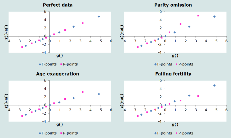
As can be seen, if older women omit live births, the P-points on the right hand of the scale (those for older ages) will drift upwards. When women report themselves (or are reported) to be older than they are, the effect is for the F-curve to curve downwards at older ages. Finally, if fertility is falling, the F-points will generally lie above the P-points.
In dealing with real data, one is often faced with a mixture of errors and trends which may be considerably more complicated than the neat archetypes set out here. Severe errors may obscure real trends and, for this reason, the method should not be applied indiscriminately.
P/F Ratios
While the P/F ratio method is not described in this manual, the ratios that result from the application of the method provide useful insights into recent trends in fertility. They can also be used as guides to the applicability of certain methods used to estimate child mortality.
Pseudo P/F ratios for each age group can be derived quite easily from a fitted relational Gompertz model. The ratio is calculated as
The numerator is the observed average parity in each age group while the denominator uses the values of α and β derived from the F-points only (much as in the F-only variant of the model) to modify the standard gompit at the mid-point of each age group. The anti-gompit is then scaled up by the level of total fertility implied by the F-points selected to be used in the model. The ratio is not calculated for the youngest age group because – typically – average parities are very low as is cumulated fertility to age 17½ , thereby causing the ratio to be unstable in that age group.
These P/F ratios can be plotted in reverse order so that the oldest age group is on the left. The series of P/F ratios can then be read as running through calendar time from left to right (since, in general, older women’s fertility will have occurred earlier in time than younger women’s fertility). Excessive deviations from the general trend suggest errors in the data. A downward trend in the P/F ratios (as plotted) shows increasing divergence between cohort and period fertility measures with increasing age, and hence is indicative of declining fertility.
Worked example
This illustration of the method uses data presented in the report on fertility from the Malawi 2008 Census. The method has been implemented in an accompanying Excel workbook.
Step 1: Calculate the reported average parities
The average parities are presented in Table 2.6 of the 2008 Malawi Census fertility report. It is not clear from the report whether the parities were edited or whether an el-Badry correction was applied to the data. The data are shown in Table 1:
Table 1 Measures of fertility from the Malawi 2008 Census
Age (at survey) | Average parity per woman | Period fertility rates |
|---|---|---|
15-19 | 0.283 | 0.111 |
20-24 | 1.532 | 0.245 |
25-29 | 2.849 | 0.230 |
30-34 | 4.185 | 0.195 |
35-39 | 5.214 | 0.147 |
40-44 | 6.034 | 0.072 |
45-49 | 6.453 | 0.032 |
Step 2: Determine the classification of the age of mother
The question on recent fertility in the 2008 Malawi Census was “how many live births in the last 12 months”. Since there is no way of dating the child’s birth, one can assume that the data are classified by age of mother at the census date rather than at the birth of her child.
Step 3: Calculate implied age-specific fertility rates
Fertility rates are presented in Table 2.6 of the 2008 Malawi Census fertility report. (The derivation of these rates, presented in Table 2.3 of the report, suggests that 5f20 was 0.250, but the rates in Table 2.6 are retained for the purpose of this example so as to allow a better comparison of the results derived.)
Step 4: Choose the standard to be applied and the model variant to be fitted
In the absence of an alternative, we apply the Booth standard, and – in order to correct the shape and level of the fertility data, elect to fit the Shape-F Level-P variant. The coefficients, e() and g(), are derived in Tables 2-4 below.
Table 2 Derivation of e(x) and g(x) when data are subject to a half-year shift
Age x | Fs(x)/F | Ys(x) | Ratio | Phi | Phi' | Phi'' | e(x) | g(x) |
|---|---|---|---|---|---|---|---|---|
[1] | [2] | [3] | [4] | [5] | [6] | [7] | [8] | [9] |
=gompit[2] | =Ys(x)/Ys(x+5) | =gompit[4] | =[5]-[6] | =[6] | ||||
14 ½ | 0.0011 | -1.9228 | 0.0094 | -1.5410 | -2.4565 | 0.9155 | -2.4565 | |
19 ½ | 0.1140 | -0.7753 | 0.3233 | -0.1216 | -1.4527 | 0.9563 | 1.3311 | -1.4527 |
24 ½ | 0.3528 | -0.0411 | 0.6007 | 0.6741 | -0.7426 | 0.9632 | 1.4167 | -0.7426 |
29 ½ | 0.5872 | 0.6305 | 0.7529 | 1.2592 | -0.0364 | 0.9530 | 1.2957 | -0.0364 |
34 ½ | 0.7800 | 1.3925 | 0.8479 | 1.8021 | 0.8405 | 0.9615 | 0.8405 | |
39 ½ | 0.9199 | 2.4830 | 0.9298 | 2.6209 | 2.1799 | 0.4409 | 2.1799 | |
44 ½ | 0.9893 | 4.5323 | 0.9893 | 4.5324 | 4.5315 | 0.0010 | 4.5315 | |
Phi’’-bar |
|
|
|
|
| 0.9575 |
|
|
Starting with the values from the standard in column [2], the gompits of the standard are calculated in column [3]. For example, in the age group ending at 19½, it is -ln(-ln(0.1140)) = -0.7753 . Note that the cumulated values apply to ages 14½, 19½ etc., reflecting the half-year shift in the classification of mothers’ ages. The ratios of successive pairs of cumulated fertility from the standard in column [2] are presented in column [4], and the gompits of these are shown in column [5]. Thus, in the age group ending at age 39½, it is 2.6209 = -ln(-ln(0.9298)) = -ln(-ln(0.9199/0.9893)).
The first and second derivatives at the point where β = 1, presented in columns [6] and [7], are evaluated using the formulae:
Finally, e(x) is derived in column [8] by differencing column [5] and [6].
Table 3 Derivation of e(x) and g(x) when data are not subject to age shifting
Age x | Fs(x)/F | Ys(x) | Ratio | Phi | Phi' | Phi'' | e(x) | g(x) |
|---|---|---|---|---|---|---|---|---|
[1] | [2] | [3] | [4] | [5] | [6] | [7] | [8] | [9] |
15 | 0.0028 | -1.7731 | 0.0204 | -1.3591 | -2.3278 | 0.9688 | -2.3278 | |
20 | 0.1358 | -0.6913 | 0.3600 | -0.0214 | -1.3753 | 0.9582 | 1.3539 | -1.3753 |
25 | 0.3773 | 0.0256 | 0.6200 | 0.7379 | -0.6748 | 0.9629 | 1.4127 | -0.6748 |
30 | 0.6086 | 0.7000 | 0.7644 | 1.3143 | 0.0393 | 0.9510 | 1.2750 | 0.0393 |
35 | 0.7962 | 1.4787 | 0.8559 | 1.8607 | 0.9450 | 0.9157 | 0.9450 | |
40 | 0.9302 | 2.6260 | 0.9378 | 2.7455 | 2.3489 | 0.3966 | 2.3489 | |
45 | 0.9919 | 4.8097 | 0.9919 | 4.8098 | 4.8086 | 0.0012 | 4.8086 | |
Phi’’-bar |
|
|
|
|
| 0.9574 |
|
|
Table 3 repeats the calculations, but for unshifted data; these values are required to produce the final, unshifted, fertility estimates. Table 4 shows the derivation of the tabulated values of e(i), g(i) and c for use with the parity data, using the parities from the standard as inputs in column [2].
Table 4 Derivation of e(i) and g(i) from parity data
Age i | Ps(i) | Ys(i) | Ratio | Phi | Phi' | Phi'' | e(i) | g(i) |
|---|---|---|---|---|---|---|---|---|
[1] | [2] | [3] | [4] | [5] | [6] | [7] | [8] | [9] |
=gompit[2] | =Ys(i)/ | =gompit[4] |
| =[5]-[4] | =[6] | |||
0 | 0.0003 | -2.0961 | 0.0056 | -1.6449 | -2.6738 | 1.0289 | -2.6738 | |
1 | 0.0521 | -1.0833 | 0.2044 | -0.4622 | -1.7469 | 0.9519 | 1.2846 | -1.7469 |
2 | 0.2549 | -0.3124 | 0.5143 | 0.4081 | -1.0159 | 0.9638 | 1.4240 | -1.0159 |
3 | 0.4957 | 0.3541 | 0.7014 | 1.0367 | -0.3349 | 0.9597 | 1.3717 | -0.3349 |
4 | 0.7067 | 1.0579 | 0.8140 | 1.5810 | 0.4406 | 1.1404 | 0.4406 | |
5 | 0.8681 | 1.9561 | 0.8969 | 2.2184 | 1.5162 | 0.7022 | 1.5162 | |
6 | 0.9679 | 3.4225 | 0.9701 | 3.4943 | 3.2238 | 0.2705 | 3.2238 | |
Phi’’-bar |
|
|
|
|
| 0.9585 |
|
|
Step 5: Evaluate the plot of P-points and F-points
Following the guidelines above, we begin by fitting models using all the P- and F-points respectively.
The results are shown in the first plot on the Diagnostic plots sheet of the accompanying Excel workbook (Figure 2):
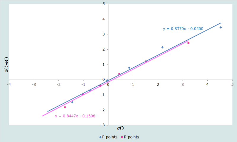
While the lines fitted to the P-points and the F-points lie almost on top of each other, neither fits their underlying data series particularly well. The F-points curve downward markedly at the oldest ages, suggesting some degree of age-exaggeration in the data, while the fact that the P-points lie just below the F-points is an indication that a slight decline in fertility is underway.
Step 6: Fit the model by selecting the points to be used
Examination of the plot suggests that a better fit to both lines might be achieved if the P- and F-points for the last age group were omitted. These points are eliminated from the plot and the resulting revised plot is re-examined (Figure 3):
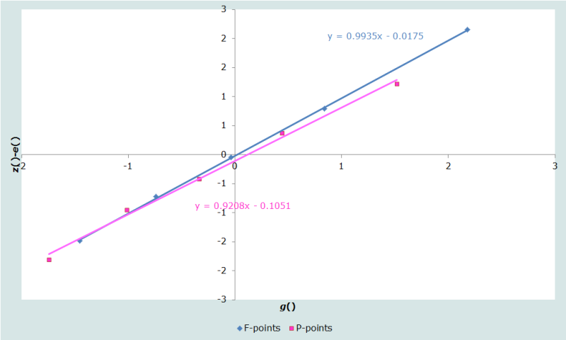
While the lines no longer lie as close together and do not remain parallel, visual inspection suggests that the removal of the next oldest P-point might cause all the remaining points to lie on a single line (Figure 4):
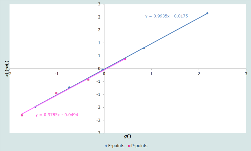
To all intents and purposes, these points can be regarding as falling on a single line, implying that the average parities and fertility rates underlying these points are consistent with each other. No evidence remains that fertility has declined. While a marginally better fit might perhaps be obtained by eliminating the P-point associated with the 35-39 age group, to further reduce the number of points included in the model in order to produce a very small improvement in the fit is not worthwhile. Indeed, the exclusion of that P-point results in a small increase in the RMSE, from 0.044 to 0.045.
We can accept this fitting of the relational Gompertz model. The third figure in the spreadsheet indicates that the equation of the straight line best fitting the remaining nine data points is z() - e()=0.9936.g() - 0.0272,
From this, the value of β is determined directly to be 0.9936, and the value of alpha is derived from the formula
where c is the average of from Table 2 for the current fertility data (since the data are subject initially to a half-year shift), and Table 4 for the parity data.
Step 7: Assess the fitted parameters
The estimated values of α (-0.0272) and β (0.9936) are comfortably close to the standard values of 0 and 1. In aggregate, the slightly negative α shows that the observed fertility distribution for Malawi in 2008 is slightly older than the standard and the value of β less than 1 suggests that the spread of the distribution is slightly wider than that of the standard.
Step 8: Fitted ASFRs and total fertility
To determine the overall level of fertility, the fitted values of α and β are applied to the standard parity gompits (column [3] of Table 4) for the age groups whose P-points were included in the model, and the anti-gompits calculated (Table 5). Dividing the observed average parities for a given age group by the fitted anti-gompit gives the level of fertility implied by the average parities (column [6] of Table 5, and an estimate of total fertility, is derived from the arithmetical average of these estimates (= 5.9784).
Table 5 Calculation of estimated total fertility , Malawi 2008 census
Age group i | Ys(i) | Y(i) | Anti-gompit | P(i) | Implied fertility level |
|---|---|---|---|---|---|
[1] | [2] | [3] | [4] | [5] | [6] |
=α + βYs(i) |
| ||||
1 | -1.0833 | -1.1034 | 0.0491 | 0.283 | 5.7662 |
2 | -0.3124 | -0.3375 | 0.2462 | 1.532 | 6.2218 |
3 | 0.3541 | 0.3246 | 0.4854 | 2.849 | 5.8694 |
4 | 1.0579 | 1.0239 | 0.6982 | 4.185 | 5.9937 |
5 | 1.9561 | 1.9162 | 0.8631 | 5.214 | 6.0407 |
T-hat |
|
|
|
| 5.9784 |
To get the associated age-specific fertility rates in conventional ages, we again apply α and β, but this time to the current fertility gompits, Ys(x), in Table 3. Taking the anti-gompit of the fitted values produces a cumulative fertility distribution. These proportions are multiplied up by the estimate of from the previous step to produce the absolute cumulated fertility distribution. Differencing and dividing by 5 produces the final age-specific fertility rates (Table 6).
Table 6 Calculation of corrected fertility rates, Malawi, 2008 Census
Age group (up to age x) | Ys(i) | Y(i) | Anti-gompit | Scaled by T-hat | ASFR |
|---|---|---|---|---|---|
[1] | [2] | [3] | [4] | [5] | [6] |
=α + β Ys(i) | F(x)=[4]*5.9784 | 5fx-5=(F(x)-F(x-5)) / 5 | |||
15 | -1.7731 | -1.7887 | 0.0025 | 0.0151 | 0.0030 |
20 | -0.6913 | -0.7140 | 0.1298 | 0.7758 | 0.1521 |
25 | 0.0256 | -0.0017 | 0.3673 | 2.1956 | 0.2840 |
30 | 0.7000 | 0.6683 | 0.5989 | 3.5807 | 0.2770 |
35 | 1.4787 | 1.4419 | 0.7894 | 4.7194 | 0.2277 |
40 | 2.6260 | 2.5817 | 0.9271 | 5.5428 | 0.1647 |
45 | 4.8097 | 4.7512 | 0.9914 | 5.9269 | 0.0768 |
50 | 13.8155 | 13.6984 | 1.0000 | 5.9784 | 0.0103 |
The ASFRs are shown in the last column of Table 6, with an implied total fertility (15-49) of 5.96 children per woman.
Detailed description of method
Introduction
The relational Gompertz model evolved from the Brass P/F ratio method. It works with the same input data, and makes use of the parity data from younger women to set the level of fertility, while the shape of the fertility distribution is determined by women’s reports on recent births.
Mathematical exposition
The relational Gompertz model of fertility, initially developed by Brass (1978), is analogous in many ways to the logit models of mortality. The model can be used to describe any fertility distribution by reference to a standard fertility distribution and the parameters used to transform it to produce the required distribution. The transformation used as a basis for the relationship between the two fertility distributions is known as the Gompertz transformation. In the original formulation of the model, it is performed on a cumulated, proportional distribution i.e. where each parity or fertility cumulant is expressed as a proportion of the total fertility rate (the summed distribution). The summed distribution therefore takes a value of one. The transformed proportions are known as gompits and are given by
where F(x) is the sum of the age-specific fertility rates cumulated to age x and F is the total fertility rate. Exactly the same relationship holds for parities, replacing F(x) with average parity for age groups, and F with the cumulated parity at age 50+. The Gompertz transformation ‘stretches’ the original age axis so that the gompits plotted against age almost form a straight line. However, the transformation is not perfect; the line tends to curve slightly at both ends, as can be seen in Figure 5, which plots the fertility rates from Booth’s (1984) standard.
The transformation can be used as a basis for a relational model because plots of the gompits of different sets of fertility rates against age tend to deviate from linearity in similar ways and, therefore, the relationship between the two such sets of gompits themselves is usually close to linear. Using the model in a relational form enables the model parameters to be estimated by fitting straight lines, which is a straightforward process and makes it simpler to interpret the results.
As the gompits of the fertility cumulants of any two fertility distributions have an approximately linear relationship, one can relate the gompits of an observed fertility distribution to the gompits of a standard distribution based on accurate data, by means of a relation
where Y(x) is the gompit of cumulated proportionate fertility at age x, and Ys(x) is the gompit of the standard fertility cumulants.
In this formulation, α represents the extent to which childbearing ages in the population differ from the standard with negative values of α making the age schedule of fertility older. β represents the extent to which the spread of childbearing differs from the spread in the standard population. The spread of the distribution is narrower for values greater than 1.
The model is, in fact, a three-parameter model. Converting the fitted gompits back to estimates of cumulative fertility using the reverse transformation produces a proportional distribution which sums to one. A third parameter is required to multiply all the fitted values up to the appropriate level of fertility. This is effectively Total Fertility – the very thing one is trying to estimate – but the estimate based on the observed data may not be reliable due to reporting errors. Thus the original fitting procedure (not described here) was adapted by Zaba (1981), whose contributions and extensions to the method is described below.
Zaba’s approach uses the gompits of the ratio of adjacent cumulants of fertility to isolate the estimation of the shape parameters from estimation of the level of fertility:
If the cumulant, F(x), conforms to a Gompertz model with parameters α and β, then
where < is the second term in the penultimate line.
For values of β close to 1, can be approximated by a Taylor series expansion about β =1:
(Equation 3)
From the definition of , .
Further, it can be shown that
(Equation 4)
Zaba (1981) evaluated this last quantity for a variety of different values of x, and showed that it is almost constant in the range 15 ≤ x < 30. (This can also be seen in Tables 2-4 where this quantity is derived). Thus, one can replace by c, the arithmetical mean of the quantities in that age range and rewrite Equation 3 as
or as
In other words, there is a linear relationship between and .
In subsequent work (Sloggett, Brass, Eldridge et al. 1994), Zaba re-expressed these terms as follows:
Term | Redefined term |
|---|---|
| g(x) |
e(x) | |
z(x) |
Hence, in this revised notation
implying a linear relationship between z - e and g.
Applying the same reasoning as above, the equivalent formulation can be derived for z(i) - e(i) in terms of α, β, c and g(i).
Variants of the fitting procedure
While the standard version of the model set out here uses data on recent fertility to determine the shape of the fertility schedule and sets the level by reference to the (selected) parity points, other variants are possible that privilege one set of input data over the other in different ways. The one presented here uses only the data on recent fertility.
The F-only variant privileges the data on recent fertility, and uses them to set both the shape and level of fertility in the model. This variant should, therefore, only be used if the analyst lacks parity data or does not wish them to influence the fit of the model. Thus, this variant simply smoothes the observed fertility rates using a relational Gompertz model.
Another extension of the relational Gompertz model that uses only the data on parity is used to estimate fertility from cohort parity increments. There is also a modified version of the relational Gompertz model making use of data from two censuses or surveys, that produces an estimate of intersurvey fertility from these data.
Construction of standards
The Booth Standard
The derivation of the Booth standard is described in detail in Booth (1984). The important aspects associated with the standard and its use in the relational Gompertz model are, first, that the standard is intended for use in medium- to high-fertility populations. Second, the standard was derived from a number of schedules produced by the Coale-Trussell fertility model, and is thus subject to the constraints imposed by that model. For the most part, these are not material.
The standard used here is not identical to that published by Booth. First, Zaba’s (1981) standard differs slightly from Booth’s below age 15 to obtain a better fit for very early patterns of childbearing. Accommodating these, it is possible to reconstruct fully the tabulated coefficients presented in Zaba (1981) and Sloggett, Brass, Eldridge et al. (1994). The standard used here is identical for the unshifted coefficients. Where the shift is required, small differences emerge, arising from the manner in which the original Booth standard has been interpolated. Zaba (1981) calculated the values for F(x + 1/2), F(x + 3/2), etc. by interpolating between successive values of F(x), F(x + 1), F(x + 2). However, as the gompit transform linearizes F(x) , it makes more sense to interpolate the gompits of F(x), Y(x) for half-year ages and then to establish the values of F(x + 1/2), F(x + 3/2) etc. by taking the appropriate anti-gompits.
Construction of alternative standards
As already noted, the Booth standard was designed for use in medium-high fertility countries. In applications of the relational Gompertz model to low-fertility countries or those with very different patterns of fertility, alternative standards are called for. We describe here briefly how to derive alternative standards.
The basic approach to constructing any standard requires a set of F(x) which can be converted by means of a gompit into a series of Y(x), and then to derive values of , and from them using the relationships established in Equations 3 and 4. From these, tabulations of z(), e() and g() can be calculated. As described above, the values of are almost constant between 15 and 30 for a given standard, and so the three values (15-19; 20-24;25-29) are averaged to produce estimates of the constant term, c.
To construct a new standard, one should begin with an accurate series of age-specific fertility rates, fs(x). Using conventional demographic analysis, we can then define the equivalent cumulants as
In most situations f(a) is not an integrable function, so numerical techniques have to be used to approximate the integral closely. Recursively, using the composite trapezium rule,
From this, the gompit, z(x) is readily calculated,
Using the properties of a Taylor expansion described in Equation 4, the components of e(x) and g(x) can be defined and expressions for these quantities derived.
The values of z(i), g(i) and e(i) are defined similarly, with the only extension being the requirement to derive the constant fertility parities associated with F(x). The parities in any given age group [x, x+n) are given by which can also be evaluated using a composite trapezium rule.
Further reading and references
Other than the source material referred to already, literature on the relational Gompertz model is sparse. While this is no doubt due in part to its being described (Booth 1984) shortly after the appearance of Manual X, a coherent exposition of how to apply the model appeared only in the SIAP manual (Sloggett, Brass, Eldridge et al. 1994). The method has been applied in numerous situations around the globe, although not in the form described here.
The PASEX suite of spreadsheets prepared by the US Census Bureau (1997), for example, offers a somewhat simplified version of the model, forcing the user to fit the straight lines to P and F using either just 2 P- points and 2 F- points, or 3 of each, with little regard for the internal consistency of the points chosen. This is the route adopted by the Malawian National Statistics Office in their analysis of fertility data from the 2008 Census. Given the high degree of consistency in these data for all women aged less than forty, the results presented in that report (TFR = 6.0) do not differ in any meaningful way from those presented in the worked example. With less-well behaved data, such congruence of results between the applications should not be taken for granted.
Booth H. 1980. "The estimation of fertility from incomplete cohort data by means of the transformed Gompertz model." Unpublished PhD thesis, London: University of London.
Booth H. 1984. "Transforming Gompertz' function for fertility analysis: The development of a standard for the relational Gompertz function", Population Studies 38(3):495-506. doi: https://dx.doi.org/10.2307/2174137
Brass W. 1978. The relational Gompertz model of fertility by age of woman. London: Centre for Population Studies, London School of Hygiene and Tropical Medicine.
Sloggett A, W Brass, SM Eldridge, IM Timæus, P Ward and B Zaba (eds). 1994. Estimation of Demographic Parameters from Census Data. Tokyo: Statistical Institute for Asia and the Pacific.
US Census Bureau. 1997. Population Analysis Spreadsheets for Excel. Washington, D.C: US Bureau of the Census. https://www.census.gov/population/international/software/pas Accessed: 17 October 2024.
Zaba B. 1981. Use of the Relational Gompertz Model in Analysing Fertility Data Collected in Retrospective Surveys. Centre for Population Studies Research Paper 81-2. London: Centre for Population Studies, London School of Hygiene & Tropical Medicine.
- Printer-friendly version
- Log in to post comments