Indirect estimation of adult mortality from data on siblings
Description of method
This method estimates adult mortality indirectly from data supplied by adults on the survival of their adult siblings (that is brothers and sisters). These data are tabulated by the age group of the respondents. Mortality can be estimated from them without requiring respondents to recall the dates when deaths occurred or the ages at death of deceased individuals. Information on the survival of brothers is used to estimate the mortality of men and information on the survival of sisters to estimate the mortality of women.
Respondents often fail to report – and may not know about - siblings who died before or during the few years after their own birth. The impact of this bias can be reduced greatly, however, by only including siblings who survived to age 15 in the analysis. In order to apply the method, a census or survey must have asked adult respondents (for example, those aged 15 to 49) how many of their sisters and/or brothers survived to the age of 15 and how many of them are still alive. Many surveys only collect information on siblings from women but data supplied by male respondents can be analysed using exactly the same methods.
Respondents’ siblings are approximately the same age, on average, as the respondents. Thus, the proportion of the siblings who survived to age 15 who are still alive is a good estimator of the conditional probability life table of surviving from age 15 to the current age of the respondents.
If mortality has changed over time, the estimated survivorship ratios reflect the mortality rates that have affected each cohort at a range of ages and dates. A ‘time location’ method has been developed that estimates how many years prior to the inquiry each cohort ratio equalled period survivorship. These intervals increase with the age of respondents, ranging from about 3 to 13 years before the collection of the data. Thus, if the survivorship ratios estimated from the reports of different age groups of respondent are translated into a common index of mortality in adulthood using a 1-parameter system of model life tables, these statistics will refer to different dates and can be used to infer the broad trend in mortality over time.
One advantage that sibling methods have over questions about household deaths is that only censuses or unusually large surveys can capture information on enough deaths in households in the year before the inquiry to yield mortality estimates that are sufficiently precise to be useful. Because respondents report on several siblings, on average, and the estimates are based on all exposure to risk at age 15 or more, estimates can be made from data on siblings in smaller inquiries. Nevertheless, all methods for the estimation of adult mortality require data on several thousand households. Moreover, the estimation procedure does not assume a population closed to migration. However, the results from the method will not be representative for small states or sub-national areas in which a substantial proportion of the population are in-migrants or have emigrated.
Data requirements and assumptions
Tabulations of data required
To estimate the mortality of adult women, respondents aged 15 to 49 should be asked how many of their sisters lived to age 15 and how many of these sisters are still alive. From tabulations of the answers to these two questions by the age group of the respondent, one can calculate:
- The proportion still alive of sisters who were alive on their 15th birthday by five-year age group of respondent. (Those who did not answer either question should be excluded from the calculations.)
To estimate the mortality of adult men, respondents aged 15 to 49 should be asked how many of their brothers lived to age 15 and how many of these brothers are still alive. From tabulations of the answers to these two questions by the age group of the respondent, one can calculate:
- The proportion still alive of brothers who were alive on their 15th birthday by five-year age group of respondent. (Those who did not answer either question should be excluded from the calculations.)
The tabulations of numbers of siblings reaching age 15 and still alive should exclude the respondent himself or herself. (Of course, this is always the case when respondents report on siblings of the opposite sex.) This requirement is explained in the discussion of the important assumptions made by the method.
Tables on respondents’ own-sex siblings (i.e. women’s sisters and men’s brothers) should be weighted only by any sample or design weights provided with the data. Tables on respondents’ opposite sex siblings (i.e. women’s brothers and men’s sisters) should be further weighted by the inverse of the number of surviving own-sex siblings of the individual respondent making the reports. This requirement is also explained in the discussion of the important assumptions made by the method.
To eliminate ambiguities related to polygynous marriage and to remarriage, interviewers in most inquiries are instructed that ‘siblings’ means children born to the same mother. Whether or not this has been done, the reports can usually be accepted as they are. So long as respondents have the same group of relatives in mind when answering the question about siblings that are still alive as they did when answering the preceding question about siblings who survived to age 15, for the purpose of estimating mortality it is immaterial exactly who their parents are.
If both men and women have been asked the relevant questions, their responses should usually be tabulated separately so that the two sets of data can be checked against each other.
Many Demographic and Health Surveys collect full sibling histories from all women aged 15 to 49. These histories ask each respondent for the name, sex, age, survival status and, if dead, age at and year of death for each of their siblings born to the same mother. All-cause death rates for men and women should usually be calculated from such histories by the direct sibling method. The reporting of recent deaths of siblings is believed to be more complete than that of more distant deaths and the direct method allows one to restrict the analysis to data on the years immediately prior to the conduct of the survey. It is straightforward, however, to determine the summary counts required by the indirect method from the full sibling histories. If reporting of siblings is fairly complete, but the reporting of the ages and dates of death of siblings is very poor, the indirect approach might yield more reliable results than the direct one.
Important assumptions
An inherent limitation of sibling-based methods for measuring adult mortality is that they underestimate mortality insofar as mortality clusters within sibships (i.e. sets of brothers and/or sisters born to the same mother). Clustering occurs whenever deaths are more concentrated in a small proportion of sibships than would be expected by chance and results from inter-sibship heterogeneity in individuals’ risk of dying (Zaba and David 1996). It causes downward bias in the mortality estimates simply because fewer members of a high mortality sibship than a low mortality sibship of the same size remain alive to answer questions about their siblings. It is impossible to correct fully for this because, at the extreme, sets of siblings whose members have all died are not reported on at all. There is no way of knowing how many of these sibships existed or what their sizes were.
Estimates of mortality trends will be biased as a result if the extent to which clustering of mortality within sibships varies with age. For example, if characteristics shared by sibs (e.g. genetic factors, early-life experiences, socio-economic status, life styles, and location) strongly influence the mortality of middle-aged adults, whereas mortality before age 40 has a large random component, estimates made for older respondents will underestimate mortality by more than those made from data supplied by younger respondents, producing a spurious impression of mortality increase over time.
The issue of bias related to multiple reporting of siblings has received substantial attention in the literature. The problem exists in survey as well as census data because the more times an individual would be reported in a census, the more likely they are to have a sibling who reports on them included in a probability sample1. Moreover, even in surveys, potential exists for multiple responses about the same individual. For example, if two daughters of the same mother are interviewed in the same household, there will be multiple reports about other members of the sibship. The standard approach to analysis used, for example, in DHS reports is based on the events and exposure time of reported siblings, leaving out the exposure time of the (surviving) respondent herself. Events and exposure time are weighted only by the respondent’s sample weight, not taking into account numbers of surviving potential respondents in the sibship.
Trussell and Rodriguez (1990) demonstrate mathematically that for groups of same-sex sibships with an identical underlying risk of dying, the standard calculation that excludes the respondent from both the denominator of the measures yields unbiased estimates of mortality. In effect, the reduction in the number of reports on dead people in the numerator that occurs because dead people cannot report on one another and the exclusion of the living respondents from the denominator offset each other precisely to give the correct risk for the sibships as a group.
The issue of the biases that could result from differential mortality by sibship size is bound up with the issue of multiple-reporting bias. It has attracted a lot of research interest because, unlike other factors that affect risk within sibships classified by sex and age of the respondent, each respondent’s sibship size is known. If mortality does not vary with sibship size, the standard estimates are the same for both every size of sibship, including one-person sibships that are excluded from the analysis because the respondent has nobody to report on, and the population as a whole. Even if mortality varies by sibship size the standard estimates remain unbiased for each sibship size, as pointed out by Masquelier (2013). To obtain mortality estimates for the population though, one must reweight the estimates for sibships of different sizes by the prevalence of sibships of that size in the population. When respondents are reporting on their own sex, one can achieve this by dividing the proportion of respondents from surviving sibships of each size by the estimated proportion of siblings surviving from age 15 to that age group in all sibships of the same size. To do this for single-person sibships, their mortality has to be estimated by extrapolation from mortality in larger sibships.
Gakidou and King (2006) argue that, instead of the standard approach, the proportions dying should be estimated for sibships that include the surviving respondent but should always be weighted in addition by the likelihood that they will be reported – that is, by the inverse of the number of potential respondents surviving in the sibship. As in Masquelier’s approach, an additional adjustment also must be made for sibships that go unreported because no member remains alive. In a multi-survey analysis of DHS full sibling histories, Obermeyer, Rajaratnam, Park et al (2010) estimate that the effect of not adjusting for the likelihood of reporting may bias overall mortality estimates downward by as much as 20 per cent. Masquelier (2013), however, argues that Obermeyer and her co-authors reweighted the data inappropriately and, as a result, exaggerated the size of any bias. He emphasizes that, if one is going to reweight, it is important only to adjust for multiple reporting by siblings who survived to the initial age from which mortality is being measured. In addition though, he questions whether the observed variation in mortality by sibship size is always real. Instead, it may well be an artefact of greater omission of dead siblings in the histories reported for large sibships. Masquelier therefore recommends using the standard approach, without attempting to reweight the data to allow for differential mortality by sibship size. This is the approach that is adopted here.
When analysing reports made on the opposite sex (for example, responses made by women about their brothers), the issues are rather different. In this case, the respondent is not a member of the group that is exposed to the risk of dying. However, the standard calculation will still give biased results for the population as a whole if the mortality of siblings of one sex is associated with the number of siblings of the opposite sex that report on them. Thus, for reports on the opposite sex a clear case exists for weighting each report by the inverse of the respondent’s number of surviving siblings of their own sex as suggested by Gakidou and King (2006). Of course, questions about siblings of the opposite sex cannot generate any information on those sibships whose members have no living siblings of the respondent’s sex. Thus, adopting this approach is equivalent to assuming that the mortality of individuals in such sibships is the same as the mortality of the rest of the population. However, in surveys that collect data from both sexes, each sex supplies this information for the other and one can further weight the deaths and exposure reported by respondents by the inverse of the probability that siblings in each age group get reported on at all.
The adult sibling method estimates the trend in mortality from data supplied by different age groups of respondent: the older the respondent, the longer ago their brothers and sisters died on average. In order to convert the series of measures of survivorship obtained indirectly from data on different age groups into a single indicator that can be compared over time, it must be assumed that the age pattern of mortality in adulthood is represented by the chosen standard life table. To estimate the time location of these measures, it is further assumed that mortality declined linearly in terms of that standard over the period being considered.
Preparatory work and preliminary investigations
Before starting the analysis, one should check how many respondents stated that they did not know how many of their siblings reached age 15 or how many of them are still alive, or who failed to answer the questions at all. Although the response rate on these questions is usually high, a few surveys have collected sufficiently incomplete data to suggest that non-response bias could be a substantial problem.
If both women and men have been asked the relevant questions, one useful check on the quality of the data on siblings is to assess how many siblings of each sex are reported, on average, by respondents of the other sex and whether the reported sex ratio at birth changes markedly as the respondents’ age increases.
One should also compare the proportions dead reported by male and female respondents of the same age. The mortality of individuals of a particular sex as reported by their brothers should equal the mortality of the same individuals as reported by their sisters. If it does not, this may indicate significant bias in the proportions dead for one or both sexes as a result of the multiple reporting of some sibships and the fact that none of the sibs have survived to report on others. Alternatively, if the proportions reported by male and female respondents diverge as their age increases, this could reflect gender differences in patterns of age misreporting or the fact that the sex that reports fewer dead siblings (usually the men) is more likely to lose touch with their families of origin and tends to assume wrongly that some of their dead siblings remain alive.
Caveats and warnings
- The original indirect sibling method was developed to estimate the survivorship of siblings from birth (Hill and Trussell 1977). Unfortunately, such reports are often very incomplete, particularly for siblings who died before or soon after the birth of the respondent. The indirect adult sibling method is recommended instead, but can only produce probabilities of surviving from age 15 to ages later in adulthood conditional on being alive at exact age 15. To produce a complete life table, one has to estimate survivorship from birth to age 15 using estimates based on another source of data.
- Deaths of siblings do not occur at one point in time but may have occurred at any time between the respondents’ 15th birthday and when they were interviewed. Therefore, applications of the indirect sibling method can only indicate the smoothed trend in adult mortality and will fail to capture short-term mortality crises or abrupt reversals in the trend in mortality such as those resulting from AIDS after the onset of a generalized HIV epidemic.
- The most up-to-date mortality estimates that can be produced using data on adult siblings are made from information supplied by respondents aged 20-24. Typically, however, only a few per cent of their brothers and sisters have died and the resulting estimates can have wide confidence intervals even in large sample surveys.
- The indirect procedure for estimating adult mortality from information on adult sibling does not involve the assumption that the population is closed to migration. Nevertheless, it can be difficult to interpret sibling-based estimates of adult mortality for sub-national geographic units, such as urban and rural areas or districts, or for respondents with particular socio-economic characteristics. This is because, although siblings usually share the same ethnic identity, many of the respondents’ siblings will live in different places from the respondents themselves and their socio-economic characteristics may differ from those of the respondents. Estimates for sub-national populations are also likely to have very large sampling errors.
Application of method
Step 1: Calculate the conditional life table survivorship ratios
The procedure for estimating life table indices from the proportions of siblings that are alive is identical no matter whether one is analysing data on brothers, sisters or siblings of both sexes and irrespective of whether the respondents are men, women or of both sexes. The accompanying Excel workbook contains panels for estimating both men’s and women’s survivorship from data on male respondents, female respondents and respondents of both sexes. Either the number of brothers or sisters alive at age 15 and the number of brothers or sisters still alive by five-year age group of respondent or the proportions of those brothers/sisters who were alive at 15 that are still alive by five-year age group of respondent should be entered into the appropriate panels. Estimates are produced from the data on respondents aged 20 to 49 years.
Survivorship is estimated between exact age 15 years and 15 + n years, where n is the upper limit of each successive age group of respondents. The following regression equation and the coefficients shown in Table 1 are used:
where 5Sn-5 represents the proportion still alive of the siblings who were alive on their 15th birthday of respondents aged n - 5 to n. For example, when n is 25, life table survivorship is estimated over the 10-year age interval from exact age 15 to exact age 25 using data on survival of siblings supplied by respondents in the age group 20-24 years.
Table 1 Coefficients for the estimation of adult survivorship from the proportions of respondents with living sisters or brothers
n | a(n) | b(n) |
|---|---|---|
25 | -0.0003 | 1.0011 |
30 | -0.1546 | 1.1560 |
35 | -0.1645 | 1.1660 |
40 | -0.1388 | 1.1406 |
45 | -0.1140 | 1.1168 |
50 | -0.1018 | 1.1066 |
Source: Timæus, Zaba and Ali (2001) | ||
Step 2: Convert the survivorship ratios into estimates of the level of mortality
To infer mortality trends from a series of survival ratios, n-15p15, obtained from different age groups of respondents and referring to different dates, it is necessary to convert them all into a common index of mortality that can be compared over time. This is done by fitting a 1‑parameter relational logit model life table to each measure and obtaining the common mortality index from the model.
A wide range of indices have been used for this purpose, including the level parameters of various systems of model life tables, survivorship ratios such as 35p15, which corresponds to the widest age range for which the adult siblings method yields measures, and life expectancy at age 15. Using the parameters of the models has the advantage of emphasizing that the full life table is being estimated by fitting a model, rather than measured directly. The measure of life expectancy summarizes survivorship across adulthood as a whole, while using survivorship avoids extrapolation into old age from measures for younger adults. Increasingly, in recent years, the estimates have been presented in terms of the probability of a 15-year old person dying before age 60, 45q15, as this measure has found favour with several international agencies as a summary indicator of the mortality of young and middle-aged adults.
In the applications of the adult sibling method presented here the survivorship ratios are converted into values of α, the level parameter of a system of relational logit model life tables, and then into estimates in these fitted models of the conditional probability of a 15-year old person dying by exact age 60 (45q15), exact age 50 (35q15) or exact age 40 (25q15). The last of these indices lies in the middle of the series of n‑15q15 values estimated using the regression models. The model life table parameter is calculated as:
where the estimates of n-15p15 come from Step 1 and the values come from a standard life table. Thus, one obtains a series of values of α corresponding to the survivorship estimates made from data on the different age groups of respondents. Higher values of α correspond to higher mortality. Then for each α,
for x = 25, 35, and 45.
The accompanying Excel workbook can calculate α and the three summary probabilities of dying using either a standard from the General family of UN Population Division (1982) model life tables or one from any of the four families of Princeton model life tables (Coale, Demeny and Vaughan 1983). The standard life table should be chosen to have an age pattern of mortality within adulthood that resembles that of the population being studied. Another life table can be used as a standard if there is reason to believe that it resembles more closely the pattern of adult mortality in the population being studied. The most suitable standard may not be the family of models that best captures the relationship between child and adult mortality. If nothing is known about the age pattern of mortality in adulthood, use of the United Nations General or Princeton West models is recommended.
Step 3: Calculate the time location of the estimates
Each survivorship ratio produced by the adult sibling survival method represents an average of the mortality prevailing during the period since the siblings’ 15th birthdays. The duration of exposure of respondents’ older siblings is longer than that of their younger siblings but averages out at about n-18.3 years (this is explained in a later section). The point of time at which the ratio equalled period survivorship depends on the level of mortality and can be estimated from the proportion of the siblings that are alive and the age of the respondents.
The only additional information required to calculate the dates to which each of the adult morality estimates refer is the date on which the inquiry that asked about the survival of brothers and sisters was conducted. This can be calculated as the average of the dates on which the interviews took place or taken as the mid-point of the period of fieldwork if exact dates of interview are not available.
The estimates are calculated as the date of fieldwork minus T, where T can be calculated for each estimate using the following equation and the coefficients in Table 2:
Table 2 Coefficients for calculating the time location of estimates of adult survivorship from the proportions of respondents with living sisters or brothers
n | a(n) | b(n) |
|---|---|---|
25 | 3.23 | 1.12 |
30 | 5.46 | 1.95 |
35 | 7.52 | 2.78 |
40 | 9.38 | 3.62 |
45 | 11.00 | 4.45 |
50 | 12.32 | 5.28 |
Source: Timæus, Zaba and Ali (2001) | ||
Worked example
This example uses data on the survival of brothers and sisters collected in the 2003 World Health Survey in Bangladesh (accessed 22th March, 2024). This survey collected data from adult men and adult women on both their brothers and sisters. The reports made by women about their sisters are used to illustrate the calculations involved in the method.
Step 1: Calculate the conditional life table survivorship ratios
The number of sisters that respondents reported as having survived to their 15th birthdays and the number of these sisters that they reported to be still alive are shown in the second and third columns of Table 3. These numbers were tabulated using the standard approach, weighting the reports only by the survey weights. The proportions alive in the fourth column are calculated by dividing the counts in the third column by those in the second column. The survivorship ratios are presented in the sixth column of Table 3. They were estimated from the proportions in the fourth column using the regression coefficients shown in Table 1. For example, for respondents aged 25-29:
Table 3 Estimation of women’s survivorship, the dates at which these estimates are located in time, and corresponding estimates of α and 25q15, from the survival of adult sisters, Bangladesh, 2003
Age group | Sisters alive at 15 | Sisters still alive | Proportion alive (5Sn-5) |
n | l (n) l(15) |
Level (α) | Probability of dying (25q15) |
Date |
|---|---|---|---|---|---|---|---|---|
15-19 | 871.6 | 851.8 | 0.9773 |
|
|
|
| |
20-24 | 858.8 | 818.7 | 0.9533 | 25 | 0.9541 | 0.517 | 0.136 | 2000.0 |
25-29 | 964.7 | 901.1 | 0.9340 | 30 | 0.9251 | 0.535 | 0.139 | 1997.7 |
30-34 | 766.9 | 702.2 | 0.9156 | 35 | 0.9031 | 0.467 | 0.128 | 1995.6 |
35-39 | 626.4 | 554.4 | 0.8850 | 40 | 0.8706 | 0.473 | 0.129 | 1993.5 |
40-44 | 552.8 | 490.7 | 0.8877 | 45 | 0.8774 | 0.226 | 0.093 | 1991.8 |
45-49 | 495.9 | 401.5 | 0.8095 | 50 | 0.7940 | 0.436 | 0.124 | 1989.9 |
Step 2: Convert the survivorship ratios into estimates of the level of mortality
The seventh column of Table 3 contains values for α, the level parameter of the system of relational logit model life tables based on a South Princeton model life table for both sexes with e0=60. The eighth column of the table contains estimates of 25q15 (the probability of a 15-year old person dying before their 40th birthday). For example, α is calculated from the estimate of 10p15 for women as:
Having calculated α, then the corresponding measure of 25q15 is:
Step 3: Calculate the time location of the estimates
The dates in the ninth column of Table 3 were calculated by subtracting the time location of the estimates from the date of the 2003 World Health Survey in Bangladesh, which was taken as 30/04/2003. The time location of each estimate is calculated from the age group of the respondents and the proportions surviving using the equations in Table 2. For example, for the first estimate of sisters’ survivorship, the calculation is:
Diagnostics, analysis and interpretation
Checks and validation
The number of respondents who stated that they did not know either how many of their siblings reached age 15 or how many of them are still alive or who did not answer the question at all should be checked before they are dropped from the analysis. If a lot of respondents failed to respond to these questions, the data supplied by those respondents who did answer them may not be representative of the population as a whole. Moreover, a high level of non-response may indicate that either the field staff or the respondents were experiencing difficulty with the questions. Thus, even when answers were supplied they may be rather unreliable. If a high level of item non-response exists, it can be illuminating to determine whether it is concentrated among a minority of field staff or a certain type of respondent.
If information about the survival of siblings has been collected from both men and women in a census or a large survey, tabulating the proportions of brothers and sisters alive separately for male and female respondents can be recommended in order to compare the consistency of their reports. While consistency of reporting does not guarantee accuracy, statistically significant differences between the proportions obtained from male or female respondents imply either that bias has been introduced into the estimates by the design of the question or that respondents of one or both sexes are answering the questions inaccurately. It is fairly common to find that male respondents report fewer siblings than female respondents and, in particular, fewer dead siblings. In other surveys, the two sexes may report similar numbers of siblings surviving to age 15 but that different numbers of them remain alive. The first type of discrepancy might result from differential age misreporting, but the second cannot.
Any bias due to clustering of mortality within families results in underestimates. Moreover, it seems unlikely that respondents invent siblings or report that their living siblings have died. Thus, the analysis should probably focus on the data for the sex that reports lower proportions of living siblings.
Interpretation
The results of the example application of the indirect adult sibling method to data from the 2003 World Health Survey in Bangladesh are portrayed graphically in Figure 1. The life table indicator presented in this instance is the probability of dying between ages 15 and 40.
The proportions of women’s sisters alive among those who lived to age 15 and of men’s brothers surviving among those who lived to age 15 were tabulated using the standard approach, weighting the reports only by the survey weights. In contrast, the equivalent proportions of men’s sisters and women’s brothers alive were tabulated after further weighting each respondent’s responses by the inverse of their number of surviving same-sex siblings.
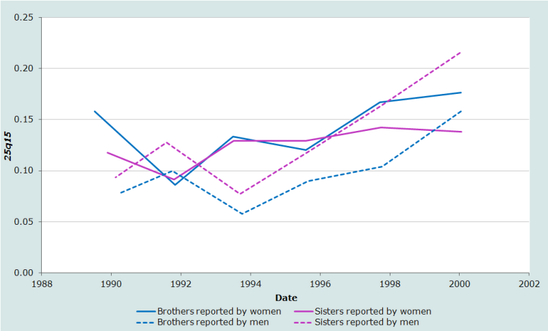
It can immediately be seen that all four series of estimates fluctuate somewhat erratically and that all four series also tend to suggest that adult mortality rose in Bangladesh during the 1990s. This seems unlikely and may suggest that the estimates made from data on older respondents are biased downward by omission of dead siblings from the reports or by other biases.
The estimates of the mortality of women (i.e. the sisters’ mortality) produced from the reports of male and female respondents indicate broadly the same level of mortality. However, the estimates of the mortality of men (i.e. the brothers’ mortality) based on the reports of male respondents indicate much lower mortality than the estimates for men based on data supplied by women. While the latter estimates suggest that the mortality of men and women in early adulthood is broadly similar, the estimates for men produced from data supplied by male respondents suggest that young men have much lower mortality than young women in Bangladesh.
Clearly these estimates are of rather poor quality. They may severely underestimate the mortality of young adults in Bangladesh. One quite plausible explanation of the apparent discrepancies between the different series of estimates is that men are more likely to omit dead siblings from their reports than women, but that downward bias resulting from clustering of mortality at the sibship level is more severe in the estimates based on the reports made by same-sex siblings than the estimates based on the reports made by opposite sex siblings. The estimates based on men’s reports about their brothers are particularly low as they suffer severely from both biases. In contrast, the two series for women appear fairly consistent because each is severely affected by one bias but less affected by the other. The implication of this pattern of errors, if it is indeed the explanation of the differences between the series, is that both sets of estimates for women probably underestimate their mortality by more than the estimates for brothers based on the reports of women. Thus, the mortality of young women in Bangladesh may well remain higher than that of men of the same age.
Detailed description of method
Introduction
The initial methods developed for estimating mortality from information on the survival of siblings were based on the idea that, on average, the ages of siblings are close to the age of a respondent. The proportion of a respondent’s siblings who are still alive is, therefore, a good estimator of life table survivorship to the age of the respondent (Hill and Trussell 1977; UN Population Division 1983). Unfortunately, field experience of this approach demonstrated that the quality of the data collected on siblings was often low because siblings who died before or shortly after the respondent’s own birth were often omitted by respondents, who may not know about them at all (Blacker and Brass 1983; Zaba 1986).
Interest in estimating mortality from data on siblings was revived by the development of the sisterhood method for measuring maternal mortality (Graham, Brass and Snow 1989). This requires data on how many sisters of the respondent survived to the age of 15, how many of them died thereafter, and whether sisters who died did so during pregnancy or within 6 to 8 weeks of the end of a pregnancy. Limiting the consideration of siblings to only those who survived to age 15 years excludes siblings who died while still young and, therefore, may have been unknown to or forgotten by the respondent. The responses supplied to the first two of these questions by respondents allow one to calculate the proportions still alive of sisters who survived to age 15 for each five-year age group. These proportions can be used to estimate the all-cause mortality of adult women. Comparable data on respondents’ brothers can be used to estimate the mortality of men.
Thus, the only information required to apply the indirect adult sibling method is summary data on the proportion of adult sisters and brothers that are still alive among those who survived to age 15 tabulated by the age group of the respondents. As the siblings are about the same age on average as the respondents, for respondents aged x, these proportions approximately equal . Because the relationship that exists between this measure and the proportion of siblings who survived to adulthood that are still alive is a close one, it can be estimated relatively precisely even in populations with unusual age patterns of mortality such as those experiencing severe HIV epidemics.
Mathematical exposition
Using the probability approach developed by Goodman, Keyfitz and Pullum (1974), Timæus, Zaba and Ali (2001) show that, in a stable population, the number of siblings ever born y years before a respondent currently aged a is given by aVy:
(Equation 1)
and
(Equation 2)
where Equation 1 gives the number of older siblings, Equation 2 the number of younger siblings, integration is over all ages at childbearing s to ω, and
z = the age of the mother at the birth of the respondent
f(z-y) = the probability of the respondents’ mothers giving birth at age z-y conditional on having given birth to the respondent at age z
r = the growth rate in a stable population.
Note that in Equations 1 and 2, f(x) is a birth distribution, which is to say the distribution of ages at giving birth of an individual woman, not the fertility distribution of the entire population.
The proportion of siblings still alive among those who lived to age 15 for respondents in a five-year age group, x to x + 5 is given by:
(Equation 3)
Calculation of the proportion of siblings alive for a given age of respondent requires a model of the birth distributions of individual women. Hill and Trussell (1977) assumed that all mothers experience the age-specific fertility rates of the general population. Thus, they could derive a sibling age distribution as a convolution of the fertility distribution. However, if women start childbearing at a wide range of ages, but compress all their childbearing into a small part of their fertile life span, as is typical in low fertility populations, one would expect the variance of the birth distribution to be considerably lower than the variance of the fertility schedule.
By contrast, when developing the sisterhood method, Graham, Brass, and Snow (1989) assumed that aVy, the distribution of age differences of siblings, could be represented by a normal distribution with a mean of zero and a variance of 80 years-squared. This assumption considerably simplifies the process of estimating the proportion of siblings who remain alive but is difficult to justify on theoretical grounds. In particular, the distribution of age differences between siblings would only be normal if the mother’s birth distribution itself was normal. Using a normal distribution for the sibling age difference distribution constitutes a reasonable approximation if the birth distribution is peaked (i.e. <35), but is less satisfactory for representing sibling age difference distributions in the case of flatter birth distributions, such as occur in high- and medium-fertility populations.
A further issue arises in growing or shrinking populations. Goldman (1978) proved that, in a growing population, an individual selected at random from those whose mothers have completed childbearing has more younger siblings ever born than older ones. The opposite is true in a shrinking population. One can understand this intuitively by considering respondents currently aged 40, all of whose mothers have completed childbearing. In a growing stable population, relatively more of these respondents will have young mothers (say those currently aged less than 65 if they have survived) than in a stationary population because, at the time of their birth, there would have been more women aged less than 25 than in the corresponding stationary population. But, if the respondents are children of young mothers, they are more likely to have younger than older siblings because their mothers have more childbearing before them than behind them.
Thus, the distribution of sibling age differences is not symmetrical: its mean lies below zero in a growing population, while the opposite is true in a shrinking population. More precisely, if the variance of the underlying birth distribution is , then the mean of the sibling age distribution lies at approximately , where r is the population growth rate. Thus, even if all women experienced the same age-specific fertility, the variance of the sibling age distribution in a growing population would still be slightly less than twice the variance of the fertility distribution and the distribution would be positively skewed. The opposite features characterize this distribution in shrinking populations.
In order to address these issues, Timæus, Zaba and Ali (2001) proposed a model of the sibling age differences that synthesized the two earlier approaches. On the basis of an investigation of the distributions of ages of older siblings reported in the birth histories collected by 12 nationally-representative surveys conducted as part of the World Fertility Survey (WFS), they concluded that the variances of birth distributions in the developing world range from about 45 to 110 years-squared. They then adapted the relational Gompertz model of fertility (Brass 1974, 1981) to represent these birth distributions, setting the β parameter in their set of models to values that vary between 1 and 1.8 to produce distributions of the appropriate width (as β increases the variance of the model distributions decreases). To allow for the absence of very short birth intervals in human populations, aV0 was set to 0 and aV1 and aV-1 to 40 per cent of the model values. The value of 40 per cent reproduces the average of the ratios aV1 / aV2 in the 12 WFS populations.
Implementation of the method
Although Equation 3 has to be evaluated numerically, in principle there is no reason it could not be solved directly for life table survivorship using the Excel Solver routine or a similar tool and a birth distribution, aVy that is appropriate for the population under study. To arrive at a unique solution, an assumption still has to be made about the age pattern of mortality within adulthood such as which standard to adopt in a 1-parameter system of model life tables. In practice, estimates are usually produced using regression models that have been fitted to simulated data on the survival of siblings generated for populations with a wide range of age structures, birth distributions and mortality schedules (Timæus, Zaba and Ali 2001). The coefficients of these models are shown in Table 1.
Mathematical exposition – time location of the estimates
Time location methods aim to estimate the time T at which the cohort measures of survival that produced the proportion of relatives surviving, , equalled the equivalent period measures, apy(T), so that:
where:
If we denote the mean time since death of those dying between y and y + a by agy, by definition:
(Equation 4)
where is the life table deaths at age z. Brass and Bamgboye (1981) show that, if mortality schedules conform to a system of 1-parameter relational logit model life tables and the trend in adult mortality is assumed to be linear in α, the parameter of that relational system of models, the time at which the cohort survivorship of adults equals period survivorship is a weighted average of the times since death of the respondents' relatives:
(Equation 5)
This time depends on the level of mortality and the ages of the relatives but is independent of the rate of change in α. Although Brass and Bamgboye’s derivation of Equation 3 takes advantage of a relationship between changes in mortality with age and with time that is specific to a relational logit system of life tables, it is possible to arrive at similar formulae for T on the basis of other reasonable assumptions about the trend in mortality with time by age (Palloni, Massagli and Marcotte 1984).
Equation 5 can be evaluated numerically, using values for avy and for the life table measures chosen on the basis of observed data. To develop a straightforward procedure for estimating T from observed characteristics of a population, a much simpler relationship must be assumed. Brass and Bamgboye (1981) argue that the change in T with a over limited age ranges is sufficiently close to linear that all respondents in a five-year age group can be treated as of the central age N. Second, they argue, at the ages and levels of mortality at which indirect methods are used to estimate adult mortality, the force of mortality increases approximately exponentially with age. As a consequence, for such applications, variation in agy with y is slight. Therefore, the weighting factors for agy in Equation 5 have little effect and all adult relatives can be treated as entering exposure at their mean age of entry, M. To a satisfactory approximation:
If survivorship in adulthood fell linearly with age, so that the same number of deaths occurred at every age, then NgM would be N/2 whatever the value of M. In less extreme life tables, mortality rises with age more rapidly than this, and the deaths of the relatives are concentrated at older ages and, therefore, in the recent portion of the N-year period. This means that the time location of the estimates is closer to the survey date than N/2. By substituting for in Equation 4 and expanding the right-hand side in powers of N, Brass and Bamgboye (1981) demonstrate that the appropriate adjustment to NgM is a function of both k and N:
(Equation 6)
Brass and Bamgboye (1981) also demonstrate that the assumption that mortality increases exponentially with age implies that in a relational logit life table system:
Solving for kN and substituting this expression into Equation 6 yields an estimate of NgM, and therefore of T, of:
Thus, in this formulation, the time references of measures of conditional survivorship obtained from data on adult relatives are estimated as half the duration of exposure, N, reduced by a factor that depends on the level of conditional survivorship relative to a standard life table.
Having arrived at this expression for T on theoretical grounds, Brass (1985) approximates NpM by 5Sx and adopts as his standard life table one in which is linear over the adult ages and is taken as (1 ‑ x/80)/2. As is linear, T = ½N and ks becomes 0. Thus, T is estimated from observed data using:
In the adult sibling method, M, the age at which exposure begins, is exactly 15 years for every sibling. The asymmetry of the sibling age difference distribution means that, in a growing population, the siblings are on average slightly younger than the respondents. This age difference varies between about zero and 1.75 years in those populations in which one is likely to want to apply the method. One can use a central value of 0.8 years in all applications. Thus, the duration of exposure, N, becomes (n - 2.5 - 0.8) - 15, where n is still the upper limit of the age group of respondents. Because M is fixed at 15 years, Equation 7 can be simplified for each age group to a linear equation of the form (Timæus, Zaba and Ali 2001):
Performance in populations with generalized HIV epidemics
The HIV epidemic poses two problems for indirect methods of estimating mortality based on the survival of relatives. First, both the sexual and vertical routes of transmission produce significant selection biases in data collected in surveys on the survival of relatives. Second, the incidence of HIV infection is concentrated among young adults. Thus, populations with significant AIDS mortality have very different age patterns of mortality both from other populations and from the model life tables used to derive coefficients for converting data on survival of relatives into measures of life table survivorship.
A major advantage of sibling methods of measuring adult mortality, compared with the orphanhood method, is that they are free of selection biases arising from direct transmission of the virus. Some residual bias due to clustering of AIDS mortality within sibships will remain. In particular, the risk of HIV infection tends to vary markedly between localities and siblings often live close to each other. The impact of this, however, will be relatively small compared with the biases that affect data that parents have supplied about their children or vice versa.
Bias in the regression coefficients used to estimate life table survivorship remains more of a problem. With respect to Equation 3, it is the change in the age pattern of mortality experienced by the siblings as a result of AIDS that is of concern, not the impact of the epidemic on the sibling age difference distribution, as the main factor shaping this distribution is the age pattern of childbearing rather than mortality or age structure.
Timæus, Zaba and Ali (2001) assess the sensitivity of the adult sibling method estimates to these problems using a combination of empirical and simulated data. They find that even in the presence of the unusual age pattern of mortality found in populations with high AIDS mortality, the adult sibling method produces estimates of survivorship that are close to the actual values. The estimates based on data on respondents aged 20-24 years and more than 40 years are extremely accurate, while those based on data for respondents aged 25 to 39 years slightly overestimate survivorship. This is because the regression coefficients fail to allow for the concentration of AIDS deaths in this age range.
To use sibling estimates of adult survivorship to monitor mortality trends, it is necessary to fit a model life table to the estimates for specific age ranges and use it to extrapolate to an index referring to a common range of ages. Somewhat surprisingly, if one converts the entire series of estimates to measures of survivorship from 15 to 50 years, 35p15, these remain fairly accurate. Those obtained from respondents aged 25 to 34 are more accurate than the estimates of on which they are based. Errors due to the failure to allow for the impact of AIDS on the mortality schedule in first calculating the coefficients and then extrapolating to a common measure of survivorship largely cancel out. This finding is robust to variation in background mortality and choice of a mortality standard. Thus, estimates of 35p15 obtained from the adult sibling method probably represent relatively robust indices for the monitoring of mortality trends as the AIDS epidemic develops. As with other indirect methods, if successive sets of data are collected for the same population, checks on the consistency of the estimates for periods when they overlap provide a powerful indication of the accuracy of the results.
Extensions and variants of the method
One can avoid some of the potential biases in cohort data on the survival of adult siblings by following up on the questions about brothers and sisters who died as adults with questions about how many of these dead siblings died less than five years ago (Masquelier et al. 2024). This enables one to estimate mortality in a clearly defined and recent period of time. Moreover, the reports on siblings who died during the last five years are likely to be more complete than those on siblings who died before then. Masquelier et al. (2024) present regression coefficients for converting sets of proportions of adult brothers or sisters who are still alive at the time of the survey, among those who were alive 5 years before, into measures of life table survivorship.
Most surveys that have collected the information required to estimate all-cause mortality of adults from data on adult siblings have also asked whether dead sisters died while pregnant or shortly after giving birth. Together these data provide the basis for applying the sisterhood method for estimating maternal mortality (Graham, Brass and Snow 1989).
It is also possible to calculate direct sibling estimates of adult mortality from the detailed sibling histories collected in many Demographic and Health Surveys and some other inquiries.
Further reading and references
The adult sibling method is not discussed in the classic manuals on indirect estimation (Sloggett, Brass, Eldridge et al. 1994; UN Population Division 1983) but is described in the United Nations manual on estimating adult mortality (UN Population Division 2002). The key reference explaining the theoretical basis of the adult sibling method and the development of the regression coefficients for conversion of proportions of surviving siblings into life table indices is Timæus, Zaba and Ali (2001). This article surveys earlier contributions to the literature.
Blacker JGC and W Brass. 1983. "Experience of retrospective enquiries to determine vital rates," in Moss, L and H Goldstein (eds). The Recall Method in Social Surveys. London: University of London Institute of Education, pp. 48-61.
Brass W. 1974. "Perspectives in population prediction: illustrated by the statistics of England and Wales", Journal of the Royal Statistical Society A137(4):532-583.
Brass W. 1981. "The use of the Gompertz relational model to estimate fertility," Paper presented at International Population Conference, Manila, 1981. Liège. International Union for the Scientific Study of Population. Vol. 3:345-362.
Brass W. 1985. Advances in Methods for Estimating Fertility and Mortality from Limited and Defective Data. London: London School of Hygiene & Tropical Medicine.
Brass W and EA Bamgboye. 1981. The Time Location of Reports of Survivorship: Estimates for Maternal and Paternal Orphanhood and the Ever-widowed. London: London School of Hygiene & Tropical Medicine.
Coale AJ, P Demeny and B Vaughan. 1983. Regional Model Life Tables and Stable Populations. London: Academic Press.
Gakidou E and G King. 2006. "Death by survey: estimating adult mortality without selection bias from sibling survival data", Demography 43(3):569-585. doi: https://dx.doi.org/10.1353/dem.2006.0024
Goldman N. 1978. "Estimating the intrinsic rate of increase of a population from the average numbers of younger and older sisters ", Demography 15(4):499-521. doi: https://dx.doi.org/10.2307/2061202
Goodman LA, N Keyfitz and TW Pullum. 1974. "Family formation and the frequency of various kinship relationships", Theoretical Population Biology 5(1):1-27. doi: https://dx.doi.org/10.1016/0040-5809(74)90049-5
Graham W, W Brass and RW Snow. 1989. "Estimating maternal mortality: The sisterhood method", Studies in Family Planning 20(3):125-135. doi: https://dx.doi.org/10.2307/1966567
Hill K and TJ Trussell. 1977. "Further developments in indirect mortality estimation", Population Studies 31(2):313-334. doi: https://dx.doi.org/10.2307/2173920
Masquelier B. 2013. "Adult mortality from sibling survival data: A reappraisal of selection biases?", Demography 50(1):207-228. doi: https://dx.doi.org/10.1007/s13524-012-0149-1
Masquelier, B, A Menashe-Oren, G Reniers, and IM Timæus. 2024. "A new method for estimating recent adult mortality from summary sibling histories." Population Health Metrics 22(32). doi: https://doi.org/10.1186/s12963-024-00350-0
Obermeyer Z, JK Rajaratnam, CH Park, E Gakidou et al. 2010. "Measuring adult mortality using sibling survival: a new analytical method and new results for 44 countries, 1974-2006", PLoS Medicine 7(4):e1000260. doi: https://dx.doi.org/10.1371/journal.pmed.1000260
Palloni A, M Massagli and J Marcotte. 1984. "Estimating adult mortality with maternal orphanhood data: analysis of sensitivity of the techniques", Population Studies 38(2):255-279. doi: https://dx.doi.org/10.1080/00324728.1984.10410289
Sloggett A, W Brass, SM Eldridge, IM Timæus, P Ward and B Zaba. 1994. Estimation of Demographic Parameters from Census Data. Tokyo, Japan: United Nations Statistical Institute for Asia and the Pacific.
Timæus IM, B Zaba and M Ali. 2001. "Estimation of adult mortality from data on adult siblings," in Zaba, B and J Blacker (eds). Brass Tacks: Essays in Medical Demography. London: Athlone, pp. 43-66. https://blogs.lshtm.ac.uk/iantimaeus/files/2012/04/Timaeus-Zaba-Ali-Siblings1.pdf
Trussell J and G Rodriguez. 1990. "A note on the sisterhood estimator of maternal mortality", Studies in Family Planning 21(6):344-346. doi: https://dx.doi.org/10.2307/1966923
UN Population Division. 1982. Model Life Tables for Developing Countries. New York: United Nations, Department of Economic and Social Affairs. https://www.un.org/development/desa/pd/sites/www.un.org.development.desa.pd/files/files/documents/2020/Jan/un_1982_model_life_tables_for_developing_countries.pdf
UN Population Division. 1983. Manual X: Indirect Techniques for Demographic Estimation. New York: United Nations, Department of Economic and Social Affairs. https://www.un.org/development/desa/pd/sites/www.un.org.development.desa.pd/files/files/documents/2020/Jan/un_1983_manual_x_-_indirect_techniques_for_demographic_estimation.pdf
UN Population Division. 2002. Methods for Estimating Adult Mortality. New York: United Nations, Department of Economic and Social Affairs, ESA/P/WP.175. https://www.un.org/development/desa/pd/sites/www.un.org.development.desa.pd/files/files/documents/2020/Jan/un_2002_methodsestimatingadultmort.pdf
Zaba B. 1986. Measurement of Emigration using Indirect Techniques: Manual for the Collection and Analysis of Data on Residence of Relatives. Liège: Ordina.
Zaba B and PH David. 1996. "Fertility and the distribution of child mortality risk among women", Population Studies 50(2):263-278. doi: https://dx.doi.org/10.1080/0032472031000149346
- Printer-friendly version
- Log in to post comments