Cohort-period fertility rates
Description of method
The availability of detailed demographic and birth history data typically collected in demographic surveys (examples being the World Fertility Surveys conducted in the 1970s, and the ongoing programme of Demographic and Health Surveys conducted by ORC Macro) has meant that – in general – direct measures of fertility estimation are to be preferred over indirect methods. Nevertheless, extensions of indirect methods to situations where there is more data can provide not only corroborating evidence to support the results derived directly, but also provide important insights into the quality of the birth history data collected.
One such extension is to apply the same logic as the Brass P/F ratio method to the birth histories, allowing a detailed investigation of the fertility data by age, period and cohort. The method yields period estimates of total fertility (TF) for either the five-year period or the two five-year periods preceding collection of the data. The method also permits the identification of common errors in the data.
Data requirements and assumptions
Tabulations of data required
- Numbers of women by age group at the survey date.
- Numbers of births by (current) age group of mother, grouped into five-year periods before the survey date. This tabulation requires, for each entry in a birth history,
- the date (month and year) of the interview;
- the child’s date of birth (month and year); and
- the mother’s current age group.
Assumptions
There is no differential fertility between women interviewed in the survey and those who have died or emigrated, and who are therefore not sampled in the survey.
Preparatory work and preliminary investigations
The method can be applied working either with the date-handling routines available in most statistical packages, or (almost as well) using dates presented in the DHS CMC format. If dates of birth and interview have not been coded as such, it is recommended that they are so coded for purposes of applying this method. The routine for doing so is described here.
Application of method
The method is applied in the following stages.
Step 1: Extract the (weighted) number of women, by age group at survey date
This is a straightforward tabulation. In the context of DHS data, women’s age group at the survey is given by the v013 variable, and the sample and design weights by v005 (divided by 106 where appropriate). The number of women in age group i is denoted by Ni = 5Nx, where x = 15, 20,…, 45 and i=x/5-2.
Step 2: Extract numbers of births by age group and period before the survey
If working with dates in CMC format, with a full birth history in a file with one record per child, the child’s current age in months is easily determined by subtracting the CMC of the child’s date of birth from the CMC of the interview date. Dividing the result by 60 and taking the integer portion of the result produces an index that allocates the child’s date of birth to successive five-year periods before the survey.
A minor modification needs to be made to accommodate the cases where the child was born in the month of interview exactly 5, 10 … years previously. Depending on the relative timing of the day of interview and the day of birth, children could be in one of two adjacent age groups. To resolve this, and to avoid allocating all such cases to one group, children in the boundary months should be allocated to age groups based on the reported day of interview, if available, and assuming that days of birth are uniformly distributed over each month. Where possible, we define b =1 if day (within the calendar month) of interview < 16 - in other words, the child’s birthday is more likely to be in the second half of the month - and 0 otherwise.
Thus
(Equation 1)
where DoI is the date of the interview and DoBc is the child’s date of birth, both recorded in CMC format. In the case of DHS data, DoI is provided by the v008 variable and DOBc by variable b3. The day of interview is given by variable v016.
A cross-tabulation (weighted, where appropriate, for the sample design) of mothers’ age group at the survey date and the grouped time of birth variable defined above is then extracted. The structure of the cross-tabulation is as shown in Table 1, where the Bi,j reflect the aggregate (weighted) number of births j years ago to women in age group i at the survey date:
Table 1 Structure of tables used to derive Cohort-Period Fertility Rates
|
| Births by period before the survey (j) | ||||
|---|---|---|---|---|---|---|
Age group of cohort at survey (i) | Number of women | 0-4 (j=0) | 5-9 (j=1) | 10-14 (j=2) | 15-19 (j=3) | 20-24 (j=4) |
15-19 (i=1) | N1 | B1,0 | B1,1 |
|
|
|
20-24 (2) | N2 | B2,0 | B2,1 | B2,2 |
|
|
25-29 (3) | N3 | B3,0 | B3,1 | B3,2 | B3,3 |
|
30-34 (4) | N4 | B4,0 | B4,1 | B4,2 | B4,3 | B4,4 |
35-39 (5) | N5 | B5,0 | B5,1 | B5,2 | B5,3 | B5,4 |
40-44 (6) | N6 | B6,0 | B6,1 | B6,2 | B6,3 | B6,4 |
45-49 (7) | N7 | B7,0 | B7,1 | B7,2 | B7,3 | B7,4 |
Note that, going back in time, the fertility rates of the youngest women will be zero for time periods in which all the women are less than 10 years old. Some births that occurred in the past will not be reported if the birth histories were collected only from women under 50.
Step 3: Derive cohort-period fertility rates based on the age group of mother at the time of the survey
If we denote age groups (or cohorts, defined by age at the survey) by the index, i, (i = 1 corresponding to the 15-19 age group, etc.) and successive five-year periods before the survey by j (j = 0 corresponding to the five-year period immediately preceding the survey, and ending at the survey date), the cohort-period fertility rate is then defined as
The ratio is divided by five because women’s exposure will be exactly five years as all women alive at the survey date must have been alive throughout each of the previous periods.
The resulting cohort-period rates present the experience of women in the same cohort (born in the same time period) in the rows, with periods in the columns, and equivalent attained ages running down the diagonals, as shown in Table 2.
Table 2 Cohort-period fertility rates, classified by age of cohort at survey
| Births by period before the survey (j) | ||||
|---|---|---|---|---|---|
Age group of cohort at survey (i) | 0-4 (j=0) | 5-9 (j=1) | 10-14 (j=2) | 15-19 (j=3) | 20-24 (j=4) |
15-19 (i=1) | f1,0 | f1,1 |
|
|
|
20-24 (2) | f2,0 | f2,1 | f2,2 |
|
|
25-29 (3) | f3,0 | f3,1 | f3,2 | f3,3 |
|
30-34 (4) | f4,0 | f4,1 | f4,2 | f4,3 | f4,4 |
35-39 (5) | f5,0 | f5,1 | f5,2 | f5,3 | f5,4 |
40-44 (6) | f6,0 | f6,1 | f6,2 | f6,3 | f6,4 |
45-49 (7) | f7,0 | f7,1 | f7,2 | f7,3 | f7,4 |
Step 4: Transpose the Cohort-Period Fertility Rates
The rates derived in Step 3 can also be classified by the age of the mother at the end of each successive five-year time period. The end of the period reflecting births that occurred in the five years before the survey date (when j = 0) is the survey date, and the end of the period 5-9 years before the survey (when j = 1) is the point exactly five years before the survey. The effect of this reclassification is that a revised series of cohort fertility indices are created:
With this reclassification, Table 2 above is rearranged as in Table 3 below. Thus, for example, the fertility of women aged 30-34 at the survey in the period 10-14 years before the survey (i.e. f4,2) would now be recast as the fertility of women who were aged 20-24 10 years before the survey (f*2,2).
Table 3 Matrix of cohort-period fertility rates, with redefined age
| Births by period before the survey (j) | ||||
|---|---|---|---|---|---|
Age group of cohort at the end of each period, k | 0-4 (j=0) | 5-9 (j=1) | 10-14 (j=2) | 15-19 (j=3) | 20-24 (j=4) |
15-19(1) | f*1,0 | f*1,1 | f*1,2 | f*1,3 | f*1,4 |
20-24(2) | f*2,0 | f*2,1 | f*2,2 | f*2,3 | f*2,4 |
25-29(3) | f*3,0 | f*3,1 | f*3,2 | f*3,3 | f*3,4 |
30-34(4) | f*4,0 | f*4,1 | f*4,2 | f*4,3 |
|
35-39(5) | f*5,0 | f*5,1 | f*5,2 |
|
|
40-44(6) | f*6,0 | f*6,1 |
|
|
|
45-49(7) | f*7,0 |
|
|
|
|
Periods further back in time will have a steadily rising number of missing values for older women if birth histories were not collected for women over 50. For example f*6,3 would represent the fertility experienced 15-19 years ago by women who were aged 40-44 exactly 15 years before the survey date. At the survey date these women would have been aged 55-59 and would not have completed the birth history section of a DHS survey.
Step 5: Derive measures of cohort fertility
Define Pk,j to be the cumulated cohort fertility (i.e. attained mean children ever born) from age 15 to the end of age group k of the cohort of women aged k at time j, then
Step 6: Derive measures of period fertility and two estimates of Total Fertility
Period fertility measures are the cumulated fertility rates in a given period. Thus, we define Fi,j to be the cumulated period fertility up to age i in period j. Hence,
Note that F7,0 is a measure of the (period) Total Fertility (TF) in the five years immediately preceding the survey. This estimate can be assumed to apply (roughly) 2½ years before the survey date.
More often than not, F7,1 cannot be evaluated directly as this would require reports of fertility among women now aged 50-54 when they were aged 45-49 in the five-year period ending five years before the survey. However, fertility in this age group is generally very low, so an approximate estimate of fertility in the period 5-9 years before the survey can be derived from
In other words, we assume that f*7,1 = f*7,0 = f7,0. If fertility has been declining, the resulting estimate will be marginally too low, but as fertility is typically very low in this age group, this bias will be unimportant.
In populations with low or moderately low fertility (current total fertility below 3 births per woman), it would be reasonable to make a similar substitution for the unmeasured fertility of women aged 40-49 exactly 10 years before the survey, as fertility in the age group 40-44 would also be low enough for small changes to impact very little on the estimated TF 10-14 years earlier. In this case we could assume that f*7,2 = f7,0 and f*6,2 = f6,1 to obtain
.
Step 7: Derive P/F ratios
The method allows the direct calculation of P/F ratios from the results produced in steps 5 and 6. The P/F ratio applicable to age group k in period j is
Thus, for example, the P/F ratio for women aged 25-29 in the five year period ending 10 years before the survey is, with k=3 and j=2 in the formulae above,
Interpretation and diagnostics
Several important interpretations arise from these results.
1. Estimates of period fertility
Step 6 showed how two estimates of fertility, applicable to points in time approximately 2½ and 7½ years before the survey, can be derived. From this, a short-term trend in fertility may be inferred.
2. Interpretation of P/F ratios and timing of the fertility decline
The P/F ratios derived in Step 7 can give insights into both the nature and timing of a decline in fertility, as well as problems with the quality of the data. The Overview of fertility estimation methods based on the P/F ratio section of the manual describes the method’s essential features.
P/F ratios of, or very close to, 1 at each age in a given period imply that there has been no change in fertility, as period and cohort measures are roughly equal. Fertility decline is indicated by P/F ratios that increase consistently with age in any given period, rising from a value close to unity for ages under 25. (25 is used because it is difficult for cohort and period fertility for the youngest cohorts to diverge too much.) Thus, if in one period before the survey, j, the P/F ratios are almost constant by age, but in the next period closer to the survey, j - 1, the P/F ratios show a clear trend with respect to age, fertility decline began (approximately) at the date dividing the two periods.
A series of low P/F ratios in a given period followed or preceded by a series of much higher P/F ratios is indicative of possible displacement of births into the period where the ratios appear low, and out of the period where the ratios appear to be uncharacteristically high. Similarly, a series of P/F ratios on a major diagonal (i.e. for a particular cohort) that departs uncharacteristically from the overall trend is indicative of age mis-statement by women, or omissions of births if the trend is observed in the oldest age group.
3. Assessment of data quality
Examination of the cohort-period fertility rates (i.e. the f*) derived in Step 4 can contribute to assessment of the quality of the data. For example, reading along the rows from right to left shows how fertility in each age group has changed as the date of the survey approached.
Since, in the absence of severe exogenous factors, the expectation is one of orderly and incremental change, deviations from orderliness may reflect reference period errors or other omissions. Three types of reference period errors are argued to be prevalent in the retrospective birth history data collected in surveys.
The first type of reference period error is that attributed to Brass who argued that older women tend to exaggerate the age of their oldest children thereby placing their birth dates further back in time than they actually occurred. This causes the level of fertility for the earliest periods preceding the survey to be over-estimated and more recent fertility to be under-estimated as births are transferred from relatively recent to more distant time periods, thereby exaggerating the apparent drop in fertility. ‘Brass effects’ are identified by the earliest cohort-period fertility rates for any age group being distinctly higher than those of slightly younger cohorts at the same attained age. This shifting of births back in time also has the effect of making fertility decline appear less than it is in reality in the more recent periods.
The second type of reference period error is that identified by Potter (1977). Women, Potter argues, have a tendency to bring earlier births closer to the date of the interview, but to report recent events correctly. This results in understatement of the level of fertility for the more distant periods preceding the survey, while recent fertility rates are correct and those in the intervening periods are exaggerated. Potter’s model is based on two propositions: first, that the “date of an event is recalled less accurately the longer ago the event took place. The second is that if a birth history is elicited by asking questions about live births in the order in which they occurred, then the date a woman attaches to any event other than the first is influenced by the information she has already given about the previous event” (Potter 1977: 341). ‘Potter effects’ are more likely to occur when women’s birth histories are collected in the order that the births occurred than when asked from youngest to oldest birth.
A third type of error of omission arises from the systematic omission of children born just before the survey, or their displacement into an earlier time period. This is brought about by the enumerator seeking to avoid asking detailed supplementary questions (for example, an anthropometry questionnaire) of children under a certain age (usually five years). Such errors have been well-documented by Cleland (1996) and Schoumaker (2010, 2011). If such omissions or displacements have occurred, the appearance of fertility decline in the period just before the survey will be exaggerated, and the P/F ratios in that most recent period will show a much greater degree of fertility decline. Some of this decline may be real, but analysts should be alert to the possible effects of this kind of omission or displacement.
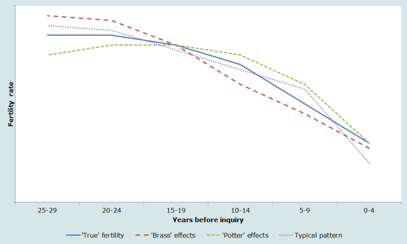
The impact of these three effects on fertility measures over time can be represented graphically, as in Figure 1.
The line marked ‘true fertility’ shows the time trend in fertility (total, or age-specific) in a hypothetical population. ‘Brass’ effects create the impression of higher fertility in the distant past and a slower fertility decline in the 10 or so years before the survey. ‘Potter’ effects produce systematic exaggerations of fertility in the 5-15 years before the survey, resulting in a mistaken impression of more rapid recent fertility decline. The ‘typical pattern’ indicates the nature of common distortions in birth history data. Fertility in the most recent period is usually too low, caused by omission (in censuses) or displacement of recent births to avoid modules on anthropometry etc. (in surveys), while fertility in the far distant past is often exaggerated (by means of ‘Brass’ effects) and visible in the apparent excess of births to very young women in many birth histories.
Worked example
The example uses retrospective birth history data collected in the 2004 Malawi Demographic and Health Survey. Tabulations have been weighted using the sample and design weights provided with the data, which accounts for the fractional women in the tabulations. The method has been implemented in an accompanying Excel workbook.
Steps 1 and 2: Extraction of data
The tabulations extracted from the DHS data files are shown in Table 4. The births reported by period before the survey have been adjusted to accommodate approximately the boundary problem discussed in the derivation of Equation 1.
Table 4 Number of women, by age group at survey, and number of births to those women, classified by timing of birth, Malawi, 2004 DHS
|
|
| Births by period before the survey (j) | ||||||
|---|---|---|---|---|---|---|---|---|---|
Age group of cohort at survey (i) | Approximate cohort birth years | Number of women | 0-4 (j=0) | 5-9 (j=1) | 10-14 (j=2) | 15-19 (j=3) | 20-24 (j=4) | 25-29 (j=5) | 30-34 (j=6) |
| 15-19 (i=1) | 1985-1989 | 2,392.0 | 713.7 | 5.2 | 0.0 | 0.0 | 0.0 | 0.0 | 0.0 |
| 20-24 (2) | 1980-1984 | 2,869.7 | 3,638.8 | 981.8 | 28.7 | 0.0 | 0.0 | 0.0 | 0.0 |
| 25-29 (3) | 1975-1979 | 2,157.4 | 2,952.3 | 2,693.6 | 859.1 | 13.6 | 0.0 | 0.0 | 0.0 |
| 30-34 (4) | 1970-1974 | 1,478.0 | 1,734.4 | 2,152.7 | 1,996.7 | 595.5 | 21.9 | 0.0 | 0.0 |
| 35-39 (5) | 1965-1969 | 1,116.8 | 1,139.6 | 1,462.6 | 1,815.5 | 1,386.4 | 508.4 | 18.1 | 0.0 |
| 40-44 (6) | 1960-1964 | 935.0 | 569.3 | 923.5 | 1,372.6 | 1,456.2 | 1,267.8 | 386.4 | 13.4 |
| 45-49 (7) | 1955-1959 | 749.1 | 235.1 | 558.8 | 952.6 | 1,024.9 | 1,128.3 | 953.3 | 311.6 |
Step 3 Derivation of cohort-period fertility rates, classified by age group of the cohort at the survey date
Table 5 shows the cohort-period fertility rates from the data in Table 4. Thus, for example, the cohort fertility rate associated with the births occurring 5-9 years to women aged 20-24 at the survey is given by .
Table 5 Cohort-period fertility rates, classified by age of mother at the survey, Malawi, 2004 DHS
| Period before the survey (j) | ||||||
|---|---|---|---|---|---|---|---|
Age group of cohort at survey (i) | 0-4 (j=0) | 5-9 (j=1) | 10-14 (j=2) | 15-19 (j=3) | 20-24 (j=4) | 25-29 (j=5) | 30-34 (j=6) |
| 15-19 (i=1) | 0.060 | 0.000 |
|
|
|
|
|
| 20-24 (2) | 0.254 | 0.068 | 0.002 |
|
|
|
|
| 25-29 (3) | 0.274 | 0.250 | 0.080 | 0.001 |
|
|
|
| 30-34 (4) | 0.235 | 0.291 | 0.270 | 0.081 | 0.003 |
|
|
| 35-39 (5) | 0.204 | 0.262 | 0.325 | 0.248 | 0.091 | 0.003 |
|
| 40-44 (6) | 0.122 | 0.198 | 0.294 | 0.311 | 0.271 | 0.083 | 0.003 |
| 45-49 (7) | 0.063 | 0.149 | 0.254 | 0.274 | 0.301 | 0.255 | 0.083 |
Step 4: Transpose the Cohort-Period Fertility Rates
The rates in Table 5 are transposed so that the rows represent equivalent attained ages at the end of each time period represented in the columns. Thus, for example, a woman aged 30-34 at the survey would have been aged 25-29 at the end of the period 5-9 years before the survey (and 20-24 at the end of the period 10-14 years before the survey), and these cohort fertility rates (0.291 and 0.270 from Table 5) are now tabulated against ages 25-29 and 20-24 respectively, as in Table 6.
Table 6 Cohort-period fertility rates, classified by age of mother at the end of each period before the survey, Malawi, 2004 DHS
| Period before the survey (j) | ||||||
|---|---|---|---|---|---|---|---|
Age group of cohort at the end of each period before the survey, k | 0-4 (j=0) | 5-9 (j=1) | 10-14 (j=2) | 15-19 (j=3) | 20-24 (j=4) | 25-29 (j=5) | 30-34 (j=6) |
| 15-19 (k=1) | 0.060 | 0.068 | 0.080 | 0.081 | 0.091 | 0.083 | 0.083 |
| 20-24 (2) | 0.254 | 0.250 | 0.270 | 0.248 | 0.271 | 0.255 | |
| 25-29 (3) | 0.274 | 0.291 | 0.325 | 0.311 | 0.301 | ||
| 30-34 (4) | 0.235 | 0.262 | 0.294 | 0.274 | |||
| 35-39 (5) | 0.204 | 0.198 | 0.254 | ||||
| 40-44 (6) | 0.122 | 0.149 | |||||
| 45-49 (7) | 0.063 | ||||||
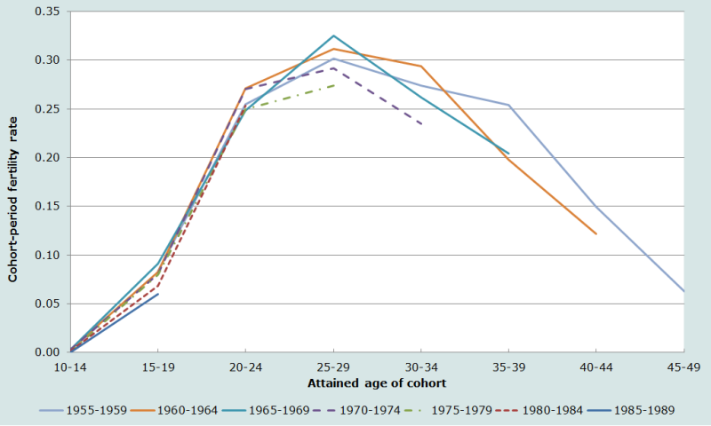
To assist with the identification of trends in fertility as well as problems or flaws in the data, the cohort-period fertility rates in Table 6 are presented graphically by birth cohort and attained age in Figure 2. There would appear to have been some generalized omission of more distant fertility in the survey as the cohort-period fertility rates for the oldest women (the 1955-59 cohort) at younger attained ages (20-24) are somewhat lower than those of slightly younger cohorts. Nonetheless, there are some indications from these data of an incipient fertility decline in Malawi in that fertility rates among the youngest cohorts (those born after 1980) are lower than those of older cohorts.
Further investigations are required to untangle these effects.
Step 5: Derive measures of cohort fertility
Cumulated cohort fertility to any given age is calculated by summing the diagonal of cohort rates in Table 6 and multiplying by 5, as shown in Table 7. Thus, for example, the cumulated cohort fertility of women aged 25-29 at the end of the period 5-9 years before the survey is given by 5(0.291 + 0.270 + 0.081) = 3.210.
Table 7 Cumulative fertility of cohorts at end of each period (P), Malawi, 2004 DHS
| Period before the survey (j) | ||||||
|---|---|---|---|---|---|---|---|
Age group of cohort at the end of each period before the survey, k | 0-4 (j=0) | 5-9 (j=1) | 10-14 (j=2) | 15-19 (j=3) | 20-24 (j=4) | 25-29 (j=5) | 30-34 (j=6) |
| 15-19 (k=1) | 0.298 | 0.342 | 0.398 | 0.403 | 0.455 | 0.413 | 0.416 |
| 20-24 (2) | 1.610 | 1.647 | 1.754 | 1.697 | 1.769 | 1.689 |
|
| 25-29 (3) | 3.015 | 3.210 | 3.322 | 3.327 | 3.195 |
|
|
| 30-34 (4) | 4.384 | 4.632 | 4.795 | 4.563 |
|
|
|
| 35-39 (5) | 5.652 | 5.783 | 5.835 |
|
|
|
|
| 40-44 (6) | 6.391 | 6.581 |
|
|
|
|
|
| 45-49 (7) | 6.895 |
|
|
|
|
|
|
Step 6: Derive measures of period fertility and two estimates of the TF
Cumulated period fertility up to a given age are derived by summing all the cohort period fertility rates (CPFRs) from Table 6 in a given column (the period) up that age, and multiplying by 5 (shown in Table 8). For example, the cumulated fertility up to age 30 in the period 5-9 years before the survey is given by 5.(0.068 + 0.250 + 0.291)=3.047.
Table 8 Cumulative fertility within periods (F), Malawi, 2004 DHS
| Period before the survey (j) | ||||||
|---|---|---|---|---|---|---|---|
Age group of cohort at the end of each period before the survey, k | 0-4 (j=0) | 5-9 (j=1) | 10-14 (j=2) | 15-19 (j=3) | 20-24 (j=4) | 25-29 (j=5) | 30-34 (j=6) |
| 15-19 (k=1) | 0.298 | 0.342 | 0.398 | 0.403 | 0.455 | 0.413 | 0.416 |
| 20-24 (2) | 1.566 | 1.591 | 1.749 | 1.644 | 1.811 | 1.686 | |
| 25-29 (3) | 2.935 | 3.045 | 3.375 | 3.202 | 3.317 | ||
| 30-34 (4) | 4.108 | 4.357 | 4.843 | 4.570 | |||
| 35-39 (5) | 5.129 | 5.345 | 6.115 | ||||
| 40-44 (6) | 5.738 | 6.091 | |||||
| 45-49 (7) | 6.051 | 6.406 | |||||
Two estimates of Total Fertility are derived. The first is that in the period 0-4 years before the survey, and is calculated directly from the data (6.1 children per woman). Fertility in the period 5-9 years before the survey is estimated by 6.091 + 5.(0.063)=6.406 children per woman.
Since the median date of interview in that DHS was November 2004, we can take the two estimates as applying to May 2002 and May 1997 respectively. The results suggest that TF fell by about 0.4 children per woman between the two periods, although displacement and omissions of most recent births may be producing an exaggerated impression of decline.
Step 7: Derive P/F ratios
P/F ratios are derived by dividing the equivalent cells in Tables 7 and 8, as shown in Table 9.
Table 9 P/F ratios, Malawi, 2004 DHS
| Period before the survey (j) | ||||||
|---|---|---|---|---|---|---|---|
Age group of cohort at the end of each period before the survey, k | 0-4 (j=0) | 5-9 (j=1) | 10-14 (j=2) | 15-19 (j=3) | 20-24 (j=4) | 25-29 (j=5) | 30-34 (j=6) |
| 15-19 (k=1) | 1.000 | 1.000 | 1.000 | 1.000 | 1.000 | 1.000 | 1.000 |
| 20-24 (2) | 1.028 | 1.035 | 1.003 | 1.032 | 0.977 | 1.002 | |
| 25-29 (3) | 1.027 | 1.054 | 0.984 | 1.039 | 0.963 | ||
| 30-34 (4) | 1.067 | 1.063 | 0.990 | 0.998 | |||
| 35-39 (5) | 1.102 | 1.082 | 0.954 | ||||
| 40-44 (6) | 1.114 | 1.080 | |||||
| 45-49 (7) | 1.139 | ||||||
It is clear from the steady increases in the P/F ratios with age in the most recent two periods that a fertility decline is under way. No such trend exists in the rations for 10-14 years before the survey. Thus, the fertility decline in Malawi appears to have started about 10 years before the survey, 1994.
The P/F ratios offer some evidence that there has been some omission or displacement of births in particular cohorts and periods. For example, the data on births occurring 10-14 years before the survey indicates P/F ratios less than one. In addition, the ratio in respect of births 10-14 years before of women then aged 20-24 (1.003) is clearly divergent from the ratio of women of the same age 5-9 years before the survey and 15-19 years before the survey. This might be attributable to rising fertility in this period, but this seems unlikely. More probably – since the ratios are too low in that period –births have been shifted into that period (possible Brass or Potter effects), thereby inflating the estimates of F and depressing the ratios. Women aged 45-49 at the survey would appear to have omitted some of their births in that in all periods 5-25 years before the survey, the P/F ratios for this cohort are lower than those of the cohort of women aged 40-44 at the survey.
Further reading and references
The method of deriving P/F ratios from survey data described here was set out in the early 1980s by Hobcraft and others (Goldman and Hobcraft 1982; Hobcraft, Goldman and Chidambaram 1982). Hobcraft, Goldman and Chidambaram (1982), in their exposition of the method, set out the approach to analysing cohort-period fertility rates by duration since marriage (and age at marriage) and duration since first birth (and age at first birth).
Beyond the sources already cited, the method has been used in a number of analyses of World Fertility Survey and DHS data. Examples include applications to Lesotho (Timæus and Balasubramanian 1984), Zimbabwe (Muhwava and Timæus 1996), West Africa (Onuoha and Timæus 1995) and Nepal (Collumbien, Timæus and Acharya 2001). Hinde and Mturi (2000) applied the method, using duration since marriage, to Tanzanian data.
Cleland J. 1996. "Demographic data collection in less developed countries", Population Studies 50(3):433-450. doi: https://dx.doi.org/10.1080/0032472031000149556
Collumbien M, IM Timæus and L Acharya. 2001. "Fertility decline in Nepal," in Sathar, ZA and JF Philips (eds). Fertility Transition in South Asia. Oxford: Oxford University Press, pp. 99-120.
Goldman N and J Hobcraft. 1982. Birth Histories. WFS Comparative Studies 17. Voorburg, Netherlands: International Statistical Institute.
Hinde A and AJ Mturi. 2000. "Recent trends in Tanzanian fertility", Population Studies 54(2):177-191. doi: https://dx.doi.org/10.1080/713779080
Hobcraft JN, N Goldman and VC Chidambaram. 1982. "Advances in the P/F ratio method for the analysis of birth histories", Population Studies 36(2):291-316. doi: https://dx.doi.org/10.2307/2174202
Muhwava W and IM Timæus. 1996. Fertility Decline in Zimbabwe. Centre for Population Studies Research Paper 96-1. London: London School of Hygiene & Tropical Medicine.
Onuoha NC and IM Timæus. 1995. "Has a fertility transition begun in West Africa?", Journal of International Development 7(1):93-116. doi: https://dx.doi.org/10.1002/jid.3380070107
Potter JE. 1977. "Problems in using birth-history analysis to estimate trends in fertility", Population Studies 31(2):335-364. doi: https://dx.doi.org/10.2307/2173921
Schoumaker B. 2010. "Reconstructing fertility trends in sub-Saharan Africa by combining multiple surveys affected by data quality problems " Paper presented at Population Association of America 2010 Annual Meeting. Dallas, TX, April 15-17, 2010.
Schoumaker B. 2011. "Omissions of births in DHS birth histories in sub-Saharan Africa: Measurement and determinants " Paper presented at Population Association of America 2011 Annual Meeting. Washington D.C., March 31 - April 2, 2011.
Timæus IM and K Balasubramanian. 1984. Evaluation of the Lesotho Fertility Survey 1977. WFS Scientific Reports, 58. Voorburg, Netherlands: International Statistical Institute.
- Printer-friendly version
- Log in to post comments