The Generalized Growth Balance Method
Description of method
Hill (1987) generalized the Brass Growth Balance method for estimating the completeness of the reporting of deaths relative to an estimate of the population on the assumption that the population was demographically stable, to non-stable populations closed to migration. This generalization can be used where one has data on the numbers by age group from two censuses and an estimate of the number of deaths by age group between the dates of the two censuses. With the additional information from two censuses it is possible to estimate age-specific growth rates in place of the constant growth rate implied by the assumption of stability. The method still assumes, however, that the proportion of deaths reported and the completeness of the census counts is the same at all adult ages and that, apart from this, the data are accurately reported. Moreover, in its common formulation it assumes that the population is closed to migration, although the method can be adapted to accommodate migration if data are available.
In all closed populations, , where the ‘partial birth’ rate, , is defined as the rate at which people turn age x in the population aged x and older and the partial death rate, , is the rate of mortality of people aged x and older. If, in this population, the deaths are under-reported to the same extent at each age then , where >is the recorded death rate for ages x and older and c is the proportion of deaths that are reported. In practice, the count of the census populations from which r(x+) is estimated may not be complete but the assumption that the undercount is the same at each age makes it possible to solve for c from the slope of the line fitted to the and data points. Mortality rates can then be estimated by dividing the numbers of deaths reported in each age group by c and dividing these numbers by an estimate of the population exposed to risk, to estimate the partial birth, growth and death rates. Moreover, as a by-product of the procedure, the less complete census counts can be adjusted to be mutually consistent, although not necessarily accurate.
Data requirements and assumptions
Tabulations of data required
- Number of women (men), by five-year age group, and for open age interval A+ (with A as high as possible), at two points in time, typically from the results of two censuses. (See the caveat below concerning the use of surveys instead of censuses.)
- Number of deaths of women (men), by five-year age group, and for open age interval A+, over the period between the two censuses or surveys
Important assumptions
- The coverage of each census is the same for all ages
- The completeness of reporting of deaths is the same for all ages above a minimum age (usually age 5 or 15)
- The population is closed to migration. Although the method can be adapted to allow for migration, accurate enough estimates of the net numbers of migrants to do so seldom exist. For national populations, net migration is often low enough to ignore, but for situations where migration is significant one needs to take this into account when interpreting results and deciding on an estimate of completeness.
Preparatory work and preliminary investigations
Before applying this method, you should investigate the quality of the data in at least the following dimensions:
- age structure of the population;
- sex structure of the population;
- age structure of the deaths; and
- sex structure of the deaths.
If the reported deaths are for a period other than that between the censuses, the numbers that would have been reported in the intercensal period need to be estimated. If one has annual vital registration data, this adjustment involves apportioning deaths in the first and last year of the period. If one has deaths reported by households the year before the dates of each of the first and second censuses, one has to estimate the numbers of deaths by interpolating between these estimates for the intercensal period (using the Estimating deaths.xlsx spreadsheet).
Caveats and warnings
In applying this method, analysts must take particular care with the following.
The interpretation and estimating processes need to take into account the source of death data (vital registration, reported by households in censuses, or recorded in hospitals) as explained below. However, the biases associated with the source of death data tend to have less impact on the estimate of completeness from the Growth Balance method than on the Synthetic Extinct Generations method.
- If applying the method to sub-national geographic areas, the issue of migration typically becomes a greater concern.
- Deciding the age range to be used to fit the straight line to the partial birth and death rates and hence estimate completeness. Issues here are: the best age to choose for the open interval if there is evidence of age exaggeration; how to accommodate data points that rise above the line at the older ages because of falling completeness possibly due to retirement-associated migration from urban to rural areas where registration is less complete; and whether to exclude ages less than either 30 or 35 because of the impact of migration which has not been allowed for specifically.
- If completeness appears to be less than 60 per cent then the uncertainty is large and this should be taken into account when interpreting the results.
- It is tempting in a situation in which census data on the age distribution of the population and household deaths are available for only one census to use in this method sample survey data on the age distribution of the population at some earlier or later date. However, for reasons that have not been adequately researched, such a combination of data sources rarely gives satisfactory results.
Application of method
Although technically one could apply this method to data in single year age categories, the data one typically works with are subject to age misstatement, so in practice one usually works with data grouped into five-year age groups. For convenience, since most data are published in this format, the spreadsheet is set up to work with data in the standard five-year groupings. However, as Blacker (1988) has shown, if this grouping fails to remove the effect of digit preference, the method should be adapted to work with an alternative five-year grouping of ages centred on, rather than starting with, ages at which heaping occurs.
Step 1: If not readily available, estimate the number of deaths reported in the period between the dates of the two estimates of the population
In the case where one has annual vital registration data, this adjustment involves apportioning deaths in the first and last year of the period to the parts of the year before and after the mean dates of fieldwork of the two inquiries. Unless the age pattern of deaths is changing very rapidly, this approximation will have no effect on the results.
If one lacks data on the number of deaths between the two inquiries but this interval falls between two periods for which one does have such estimates (for example, because each inquiry included a question about deaths in the household during the previous year), one can use the Estimating deaths spreadsheet. This spreadsheet estimates the number of deaths between two points in time given estimates of deaths over two other periods. To use this spreadsheet, you need the number of deaths divided into five-year age groups for two periods (periods 1 and 2), the start and end dates for each of these periods, and the start date and end date of the period for which one wishes to estimate the number of deaths.
Step 2: Cumulate population, deaths and migrants downwards
To estimate partial birth, death (and migration) rates one needs to cumulate the numbers in the population, and the number of deaths (and the net number of migrants) for ages x and older. Thus, in the case of the population the following equation is used:
where A is the age at the start of the open age interval.
Analogous equations are used to calculate the number of deaths aged x and older, D(x+). In the case where these are available (unlikely though this may be) analogous equations can be used to calculate the net number of migrants aged x and older, NM(x+)). Where the numbers of migrants is not known this column is set to zero (or left blank) and the method is applied taking into account this omission, as described below.
Step 3: Calculate the person-years of life lived, PYL(x+)
In order to estimate partial birth and death rates (and if one has data on the net numbers of migrants, migration rates) one needs to estimate the person-years of exposure. This is estimated using the following formula:
where t1 is the time of the first census, and t2 the time of the second census.
Step 4: Calculate the number of people who turned x in the population, N(x)
The number of people who turned x (i.e. were ‘born’ into the open age interval x+) in the population is estimated as the geometric mean of the numbers in a cohort at times t1 and t2 divided by 5, multiplied by the length of the period between the censuses, in years, using the following formula:
Step 5: Calculate partial birth and death rates, b(x+) and d(x+), and partial growth rate r(x+) corrected for migration, i(x+)
The partial birth and death rates are estimated using the following formulae:
while the partial growth rate less the partial migration rate is calculated using the following formula:
Step 6: Plot graph of b(x+) - r(x+) + nm(x+) against d(x+), and examine to decide on the range over which the line should be fitted
Start by setting the lower age to 5 and the upper age to A-1, where A is the age at the start of the open interval of the data. Inspect the diagnostic plots and decide on the age interval over which the line is to be fitted. If there is greater age exaggeration in ages at death than in ages of the living the points plotted to the right (older ages) will fall progressively below the line with age. This indicates that a lower maximum age is called for – stepping down in five-year steps until the effect is removed. Also, if the absolute value of the residuals of the end points are too large (e.g. exceed 0.01) then the maximum age should be lowered to prevent these points unduly influencing the slope of the line. If the age exaggeration is the same in the population and the deaths then this will have no effect on the slope and hence the estimate of completeness of reporting, but the age-specific death rates will be biased downward for these ages.
If the points plotted at the younger ages (left-hand side), particularly ages 15 to 30, deviate noticeably from the straight line and one has not included any data on migration, this probably indicates that there is significant migration (unless there is age differential under-enumeration). One should thus increase the lower age of the age interval used to fit the line to age 30 or 35, depending on which produces the most sensible fit to the data.
Step 7: Fit line and estimate completeness, c
In order to estimate the completeness of reporting of deaths relative to the population, one starts by plotting b(x+)-r(x+)+i(x+) against d(x+) and estimating the coefficients of the straight line fitted to these points, using orthogonal regression, as follows:
and
where b is the slope of the line and a the intercept, and the yi represent the b(x+) - r(x+) + i(x+), the xi represent the d(x+) and and represent the means of the two series, respectively.
After fitting the straight line to all the points, one inspects the plotted points relative to the line and the residuals in order to decide on the best range of ages to use to determine the completeness of reporting of deaths. How one decides this is discussed in more detail below but any residuals greater than 1 per cent in absolute value should be excluded. A line is then fitted to these points, from which new values of a and b are determined. As a general rule, it is not recommended to truncate at an age ending in zero in a population with significant digital preference.
The completeness of reporting of deaths, c, is derived from the values of a and b as follows. Since
and
We estimate c by assuming the larger of k1 and k2 equals 1. Thus, if , assume that k2 = 1 and hence
,
and, if , assume that k1 = 1 and hence
).
Then c is calculated as follows:
.
Step 8: Estimate mortality rates adjusted for incompleteness of reporting of deaths
In order to compute mortality rates one needs first to correct the census population for relative under-enumeration. This is achieved by dividing the numbers from the first census by k1 and the numbers from the second census by k2.
Next one needs to adjust the number of deaths for incompleteness by dividing the reported number of deaths by the estimate of completeness, c.
The adjusted person-years of exposure, PYLa(x,5), are estimated in the same way as before but using the population corrected for under-enumeration as follows:
Next one needs to adjust the number of deaths for incompleteness by dividing the reported number of deaths by the estimate of completeness, c, and dividing this by PYLa(x,5) to produce mortality rates adjusted for the incompleteness of the reporting of deaths as follows:
Note that technically one could drop the k1/k2 adjustment and still get the same estimates of the mortality rates (since the same adjustment is made to both the numerator and the denominator). However, in that case the estimate of completeness is relative to the average of the census populations ignoring the fact that one is undercounted relative to the other.
Step 9: Smooth using relational logit model life table
Because the age-specific rates can be quite erratic they need to be graduated (smoothed). This can be achieved by fitting a Brass relational logit function to a sex-specific standard life table which is considered to have the same shape as that generated by the mortality rates of the population being investigated.
The accompanying workbook contains a spreadsheet that allows one to produce a smooth set of mortality rates by using a relational logit model fitted to the life table generated by the adjusted mortality rates. The user can choose between the standard from the General family of United Nations model life tables or one from any of the four families of Princeton model life tables. The logit transforms of these tables together with a model life table of a population experiencing an AIDS epidemic (Timæus 2007) appear in the Models sheet. This spreadsheet also allows the user to input logit transforms of an alternative life table if there is reason to assume that it has a similar pattern of adult mortality to that of the population being studied.
In order to fit the model, probabilities of people aged x dying in the next 5 years, 5qx, are estimated from the adjusted rates of mortality as follows:
From this the life table with a radix of l5 = 1 is calculated as follows:
The coefficients, α and β are determined by fitting the relational logit model as follows:
where and superscript ‘s’ designates values based on a standard life table.
The fitted life table is then generated from the standard life table using the coefficients α and β as follows:
and
The smoothed mortality rates are derived from this life table as follows:
and
where i.e. and ω is the age above which the life table has no more survivors.
Worked example
This example uses data on the numbers of males in the population from the South African Census in 2001 and the Community Survey in 2007, on number of deaths from vital registration for the years 2001 to 2007, and on the net number of migrants estimated from the change in foreign-born counted in the two surveys, less an estimate of the number of South Africans who emigrated between the two surveys. The example appears in the GGB South Africa_males workbook.
Step 1: If not readily available, estimate the number of deaths reported in the period between the dates of the two estimates of the population
The registered deaths for the years 2001 to 2007 for South African males are given in Table 1.
Table 1 Calculation of deaths between census dates, South African males, 2001-2007
Age | 2001 | 2002-2006 | 2007 | Total between censuses |
|---|---|---|---|---|
0-4 | 29,005 | 186,346 | 40,314 | 197,912 |
5-9 | 2,118 | 14,733 | 2,854 | 15,566 |
10-14 | 1,745 | 10,535 | 2,233 | 11,207 |
15-19 | 4,470 | 23,857 | 4,860 | 25,473 |
20-24 | 8,931 | 51,588 | 10,875 | 54,960 |
25-29 | 16,834 | 96,705 | 18,405 | 102,802 |
30-34 | 20,892 | 137,355 | 28,245 | 145,588 |
35-39 | 21,068 | 137,502 | 29,258 | 145,900 |
40-44 | 19,322 | 128,217 | 26,973 | 135,936 |
45-49 | 17,881 | 113,891 | 24,761 | 121,010 |
50-54 | 16,883 | 104,508 | 22,790 | 111,157 |
55-59 | 14,544 | 90,919 | 21,317 | 96,854 |
60-64 | 15,097 | 84,351 | 17,410 | 89,930 |
65-69 | 13,011 | 77,680 | 17,878 | 82,843 |
70-74 | 14,035 | 68,147 | 13,771 | 73,036 |
75-79 | 10,846 | 59,859 | 12,534 | 63,871 |
80-84 | 9,161 | 44,986 | 8,872 | 48,163 |
85+ | 7,602 | 43,233 | 10,009 | 46,196 |
The reference time for the census in 2001 was midnight between 9 and 10 October 2001. The Community Survey took place over a number of weeks in February so we can assume a reference time of midnight between 14 and 15 February 2007. Thus, if we assume deaths occur uniformly over the respective calendar years, we can apportion the deaths in 2001 and in 2007 and add these to the total for the years 2002 to 2006 to get the total number of deaths between the two estimates of the population. For example, for the age group 20-24 the number is calculated as follows:
Step 2: Cumulate population, deaths and migrants downwards
One accumulates the numbers in the population, deaths and migrants from the oldest age downwards (Table 2).
Table 2 Calculation of the cumulated populations, deaths and migrants, South African males, 2001-2007
Age | 5Nx(t1) | 5Nx(t2) | 5Dx | 5NMx | P1(x+) | P2(x+) | D(x+) | NM(x+) |
|---|---|---|---|---|---|---|---|---|
0 | 2,223,006 | 2,505,744 | 197,912 | 10,605 | 21,434,045 | 23,348,679 | 1,568,404 | 128,946 |
5 | 2,425,066 | 2,560,642 | 15,566 | 2,848 | 19,211,039 | 20,842,935 | 1,370,492 | 118,341 |
10 | 2,518,985 | 2,452,339 | 11,207 | 5,153 | 16,785,973 | 18,282,293 | 1,354,926 | 115,492 |
15 | 2,453,156 | 2,553,293 | 25,473 | 16,574 | 14,266,988 | 15,829,955 | 1,343,719 | 110,339 |
20 | 2,099,417 | 2,362,519 | 54,960 | 14,803 | 11,813,832 | 13,276,662 | 1,318,246 | 93,766 |
25 | 1,899,275 | 2,033,165 | 102,802 | 4,714 | 9,714,415 | 10,914,143 | 1,263,286 | 78,963 |
30 | 1,594,624 | 1,875,483 | 145,588 | 13,331 | 7,815,140 | 8,880,977 | 1,160,484 | 74,249 |
35 | 1,441,657 | 1,548,185 | 145,900 | 9,693 | 6,220,516 | 7,005,495 | 1,014,896 | 60,918 |
40 | 1,233,813 | 1,306,900 | 135,936 | 7,464 | 4,778,859 | 5,457,310 | 868,996 | 51,225 |
45 | 967,744 | 1,104,294 | 121,010 | 8,719 | 3,545,046 | 4,150,410 | 733,060 | 43,761 |
50 | 769,627 | 888,042 | 111,157 | 9,413 | 2,577,302 | 3,046,116 | 612,050 | 35,042 |
55 | 552,402 | 708,812 | 96,854 | 4,640 | 1,807,675 | 2,158,074 | 500,893 | 25,629 |
60 | 444,592 | 491,871 | 89,930 | 5,081 | 1,255,273 | 1,449,261 | 404,039 | 20,989 |
65 | 304,835 | 394,305 | 82,843 | 4,922 | 810,681 | 957,391 | 314,108 | 15,908 |
70 | 232,604 | 241,976 | 73,036 | 4,334 | 505,846 | 563,086 | 231,266 | 10,986 |
75 | 136,466 | 163,112 | 63,871 | 2,980 | 273,242 | 321,110 | 158,229 | 6,652 |
80 | 90,856 | 87,698 | 48,163 | 1,662 | 136,776 | 157,998 | 94,359 | 3,672 |
85 | 45,920 | 70,299 | 46,196 | 2,009 | 45,920 | 70,299 | 46,196 | 2,009 |
Step 3: Calculate the person-years of life lived, PYL(x+)
Calculating person-years lived requires an estimate of the time between the two counts. This has been calculated using the YEARFRAC function in Excel on the basis of the date of the day following the time reference for the censuses. Counting days and dividing by 365 produces a slightly different estimate (5.3507 years) but has a negligible impact on the estimate of completeness.
The person-years of life lived is given in column 2 of Table 3 and is calculated from the numbers of the cumulated population in columns 2 and 3 of Table 2. For age 20, for example, as follows:
Table 3 Calculation of the cumulated populations, deaths and migrants, South African males, 2001-2007
Age | PYL(x+) | N(x) | b(x+) | r(x+)-i(x+) | d(x+) = X | b(x+)-r(x+) +i(x+) = Y | a+bx | Residuals y-(a+bx) |
|---|---|---|---|---|---|---|---|---|
0 | 119,775,275 |
|
| #N/A | 0.00000 |
| -0.0047 |
|
5 | 107,136,837 | 2,554,810 | 0.02385 | 0.01413 | 0.01279 | 0.00972 | 0.0093 | 0.0004 |
10 | 93,793,458 | 2,611,355 | 0.02784 | 0.01472 | 0.01445 | 0.01312 | 0.0111 | 0.0020 |
15 | 80,461,835 | 2,715,670 | 0.03375 | 0.01805 | 0.01670 | 0.01570 | 0.0135 | 0.0022 |
20 | 67,053,861 | 2,577,889 | 0.03845 | 0.02042 | 0.01966 | 0.01803 | 0.0168 | 0.0013 |
25 | 55,129,886 | 2,212,329 | 0.04013 | 0.02033 | 0.02291 | 0.01980 | 0.0203 | -0.0005 |
30 | 44,604,915 | 2,020,991 | 0.04531 | 0.02223 | 0.02602 | 0.02308 | 0.0237 | -0.0006 |
35 | 35,344,071 | 1,682,498 | 0.04760 | 0.02049 | 0.02871 | 0.02712 | 0.0266 | 0.0005 |
40 | 27,342,320 | 1,469,826 | 0.05376 | 0.02294 | 0.03178 | 0.03082 | 0.0300 | 0.0008 |
45 | 20,537,160 | 1,249,916 | 0.06086 | 0.02735 | 0.03569 | 0.03352 | 0.0343 | -0.0007 |
50 | 15,001,678 | 992,684 | 0.06617 | 0.02891 | 0.04080 | 0.03726 | 0.0398 | -0.0026 |
55 | 10,574,924 | 790,897 | 0.07479 | 0.03071 | 0.04737 | 0.04408 | 0.0470 | -0.0029 |
60 | 7,221,483 | 558,171 | 0.07729 | 0.02396 | 0.05595 | 0.05334 | 0.0564 | -0.0030 |
65 | 4,716,866 | 448,343 | 0.09505 | 0.02773 | 0.06659 | 0.06732 | 0.0680 | -0.0006 |
70 | 2,857,463 | 290,826 | 0.10178 | 0.01619 | 0.08093 | 0.08559 | 0.0836 | 0.0020 |
75 | 1,585,932 | 208,577 | 0.13152 | 0.02599 | 0.09977 | 0.10553 | 0.1041 | 0.0014 |
80 | 787,071 | 117,144 | 0.14884 | 0.02230 | 0.11989 | 0.12654 | 0.1261 | 0.0005 |
85 | 304,201 |
|
|
|
|
|
|
|
Step 4: Calculate the number of people who turned x in the population, N(x)
The numbers of people who turned x are shown in the third column of Table 3. For example, the number who turned 20 is estimated from the population numbers in columns 2 and 3 of Table 1 as follows:
Step 5: Calculate partial birth and death rates, b(x+) and d(x+), and partial growth rate r(x+) corrected for migration, i(x+)
The partial birth and death rates are shown in columns 4 and 6 of Table 3. The partial birth and death rates are calculated from the partial births (column 3 of Table 3) and the partial deaths (column 8 of Table 2) as follows for age 20, for example:
The partial growth rate less the partial net in-migration rate is shown in column 5 of Table 3 and is calculated for age 20, for example, using the cumulated populations given in columns 2 and 3 of Table 3 and cumulated net in-migration given in the last column of Table 2 as follows:
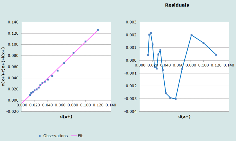
Step 6: Plot graph of b(x+)-r(x+)+i(x+) against d(x+), and examine to decide on the range over which the line should be fitted
In order to plot the graph and fit the line to all of the data points, one starts by setting the lower age to 5 and the upper age to 84 (since the open interval for these data is 85+). The values of b(x+) - r(x+) + i(x+) plotted against d(x+) are shown in Figure 1.
Inspection of the diagnostic plots in Figure 1 suggests that the points lie fairly close to the fitted straight line, indicating that there is little migration which has not been accounted for. Thus there is little reason to alter the age range over which the line is fitted. Thus, as might be expected, increasing the minimum age has very little effect on the estimate of completeness of 91 per cent. Likewise, even though the results may be affected to some extent by a falling off of completeness at the older ages (see the application of the Synthetic Extinct Generations method to these data), the estimate is little changed by excluding the last or the last two points (i.e. reducing the upper age of age interval used to fit the data). Dropping further points, however, increases completeness to implausible levels which suggests that the data (probably the population data) are far from perfect.
Step 7: Fit line and estimate completeness, c
The coefficients of the straight line fitted to the points in Figure 1 are estimated as follows:
The relative completeness of enumeration of the census populations is estimated as follows:
Thus k2 > k1 and so we assume k2 = 1 and hence k1 = 0.9753 (i.e. the first population is undercounted relative to the second by some 2.5 per cent).
The completeness of reporting of deaths, c, is 91 per cent (relative to the 2007 count), calculated as follows:
Step 8: Estimate mortality rates adjusted for incompleteness of reporting of deaths
The adjusted population as at the first census date is the enumerated population given in column 2 of Table 2 divided by k1. For example the adjusted population for age 20 is
The adjusted population at the second census date is the enumerated population given in column 3 of Table 2 divided by k2. Since, by assumption, k2 = 1, these numbers are the same as those given in column 3 of Table 2.
Next the deaths are adjusted for incompleteness by dividing the number of reported deaths in each age group shown in column 4 of Table 2 by the estimate of completeness. These numbers are shown in column 4 of Table 4. For example, for age 20 the number is derived from the number of reported deaths, 54 960, as follows:
The adjusted person-years of life lived (column 5 of Table 4) is the geometric average of the populations in columns 2 and 3 of Table 4 multiplied by the length (in years) of the period between the censuses, which in this case is 5.3541 years. For age 20 this is
The mortality rates adjusted for incompleteness of reporting of deaths (column 6 of Table 4) are derived by dividing the adjusted deaths by the adjusted person-years of life lived. For example, for the 20-24 age group the adjusted rate is calculated as follows:
Table 4 Calculation of adjusted mortality rates, South African males, 2001-2007
Age | Adjusted 5Nx(t1) | Adjusted 5Nx(t2) | Adjusted 5Dx | Adjusted PYL(x,5) | Adjusted 5mx |
|---|---|---|---|---|---|
0 |
|
|
|
|
|
5 | 2,486,532 | 2,560,642 | 17,193 | 13,510,001 | 0.0013 |
10 | 2,582,831 | 2,452,339 | 12,378 | 13,474,797 | 0.0009 |
15 | 2,515,334 | 2,553,293 | 28,134 | 13,568,508 | 0.0021 |
20 | 2,152,629 | 2,362,519 | 60,701 | 12,074,140 | 0.0050 |
25 | 1,947,414 | 2,033,165 | 113,541 | 10,653,675 | 0.0107 |
30 | 1,635,041 | 1,875,483 | 160,796 | 9,375,725 | 0.0172 |
35 | 1,478,197 | 1,548,185 | 161,141 | 8,099,564 | 0.0199 |
40 | 1,265,085 | 1,306,900 | 150,136 | 6,884,383 | 0.0218 |
45 | 992,273 | 1,104,294 | 133,651 | 5,604,563 | 0.0238 |
50 | 789,134 | 888,042 | 122,768 | 4,482,045 | 0.0274 |
55 | 566,403 | 708,812 | 106,972 | 3,392,442 | 0.0315 |
60 | 455,861 | 491,871 | 99,325 | 2,535,277 | 0.0392 |
65 | 312,561 | 394,305 | 91,497 | 1,879,609 | 0.0487 |
70 | 238,500 | 241,976 | 80,666 | 1,286,217 | 0.0627 |
75 | 139,925 | 163,112 | 70,543 | 808,863 | 0.0872 |
80 | 93,159 | 87,698 | 53,194 | 483,940 | 0.1099 |
85 | 47,084 | 70,299 | 51,021 | 308,032 | 0.1656 |
Step 9: Smooth using relational logit model life table
Estimates of probabilities of people aged x dying in the next 5 years, 5qx, estimated from the adjusted rates of mortality which appear in column 6 of Table 4, are shown in the second column of Table 5. For example, the probability of a 20-year old woman dying before reaching age 25 is calculated as follows:
The life table proportions of five-year olds alive at age x+5 estimated from the proportion alive at age x using these values appear in column 3 of Table 5. For example, the proportion alive at age 25 is calculated as follows:
Table 5 Calculation of smoothed mortality rates using a relational logit model life table, South African males, 2001-2007
Age | 5qx | lx/l5 | Obs. Y(x) | AIDS Cdn. ls(x) | Cdn. Ys(x) | Fitted Y(x) | Fitted l(x) | T(x) | Smooth 5mx |
|---|---|---|---|---|---|---|---|---|---|
0 |
|
|
|
|
|
|
|
|
|
5 | 0.0063 | 1 |
| 1.0000 |
|
| 1 | 50.898 | 0.0032 |
10 | 0.0046 | 0.9937 | -2.5270 | 0.9785 | -1.9081 | -2.0574 | 0.9839 | 45.739 | 0.0030 |
15 | 0.0103 | 0.9891 | -2.2542 | 0.9632 | -1.6326 | -1.7297 | 0.9695 | 40.856 | 0.0025 |
20 | 0.0248 | 0.9789 | -1.9186 | 0.9512 | -1.4853 | -1.5545 | 0.9573 | 36.039 | 0.0043 |
25 | 0.0519 | 0.9546 | -1.5229 | 0.9324 | -1.3120 | -1.3485 | 0.9368 | 31.303 | 0.0090 |
30 | 0.0822 | 0.9051 | -1.1273 | 0.8969 | -1.0818 | -1.0747 | 0.8956 | 26.722 | 0.0159 |
35 | 0.0948 | 0.8306 | -0.7951 | 0.8420 | -0.8365 | -0.7829 | 0.8272 | 22.415 | 0.0206 |
40 | 0.1034 | 0.7519 | -0.5544 | 0.7794 | -0.6311 | -0.5386 | 0.7460 | 18.482 | 0.0241 |
45 | 0.1125 | 0.6742 | -0.3636 | 0.7148 | -0.4593 | -0.3344 | 0.6612 | 14.964 | 0.0244 |
50 | 0.1282 | 0.5983 | -0.1992 | 0.6560 | -0.3228 | -0.1720 | 0.5851 | 11.848 | 0.0234 |
55 | 0.1461 | 0.5216 | -0.0433 | 0.6048 | -0.2127 | -0.0410 | 0.5205 | 9.084 | 0.0258 |
60 | 0.1784 | 0.4454 | 0.1097 | 0.5530 | -0.1064 | 0.0854 | 0.4574 | 6.640 | 0.0337 |
65 | 0.2170 | 0.3659 | 0.2749 | 0.4918 | 0.0163 | 0.2313 | 0.3864 | 4.530 | 0.0503 |
70 | 0.2711 | 0.2865 | 0.4562 | 0.4119 | 0.1781 | 0.4237 | 0.3000 | 2.814 | 0.0717 |
75 | 0.3580 | 0.2089 | 0.6659 | 0.3178 | 0.3819 | 0.6661 | 0.2088 | 1.542 | 0.1008 |
80 | 0.4311 | 0.1341 | 0.9327 | 0.2173 | 0.6408 | 0.9740 | 0.1248 | 0.708 | 0.1470 |
85 | #N/A | 0.0763 | 1.2470 | 0.1201 | 0.9959 | 1.3964 | 0.0577 | 0.252 | 0.2081 |
The logit transformations of the proportions surviving appear in column 4 of Table 5. For example, the logit transformation of the l20 is calculated as follows:
The logit transformation of the conditional life table for males based on the AIDS life table with e0=50 in column 5 of Table 5 appears in column 6 of Table 5. As can be seen from Figure 2, the AIDS model does not fit the data particularly well, but fits better than any table which does not reflect the impact of HIV on mortality.
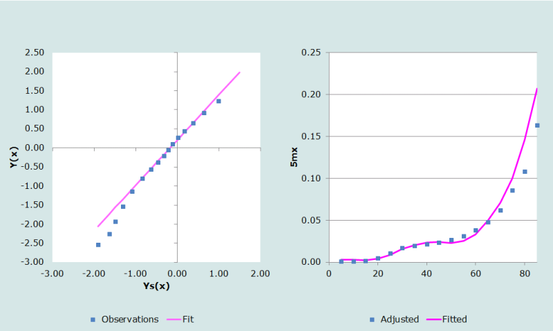
The coefficients, α and β are determined as the intercept and slope of the straight line fitted to the logit transformations in columns 4 and 6 of Table 5 over the range of ages chosen by the user (45 and 80 in this example), namely 0.2119 and 1.1893 respectively.
These coefficients are then applied to the logit transformation of the conditional model life table to produce the fitted logits in column 7 of Table 5. Thus, for example, the fitted logit at age 20 is calculated as follows:
These values are then used to produce the fitted life table in column 8 of Table 5. For example, the value at age 20 is calculated as follows:
The conditional years of life lived, Tx, which appear in column 9 of Table 5 are then calculated from the fitted life table and these numbers are then used to produce the smoothed mortality rates which appear in column 10 of Table 5. For example, for age 80
Diagnostics, analysis and interpretation
Checks and validation
The estimate of completeness is 91 per cent. The first check on this result is a comparison with the results for the opposite sex. For example, applying the same method as described above for men to the data for women during the same period (GGB_South Africa_females) gives an estimate of completeness of 89 per cent. Past research (Dorrington, Moultrie and Timæus 2004) leads to the expectation that the estimates should be similar, so the results are sufficiently close to validate the estimates.
A second check on the results is to compare them with the result from the Synthetic Extinct Generations method (SEG_South Africa_males), which estimated the completeness of death reporting over the age range 5 to 84 to be 94 per cent, which is also sufficiently close to validate the results.
A third check is to compare estimates of various key indicators of mortality with those from other sources, such as previous estimates for the country or the World Population Prospects (UN Population Division 2011). The estimate of 45q15 from the observed mortality rates after adjusting for incompleteness is 52.3 per cent, while the estimate of 45q15 from the WPP for the period 2000-2005 is 52.8 per cent, again suggesting little reason to question the results.
As a matter of interest, application of the Brass Growth Balance method to these data (estimating the population in the middle of the period as the average of the two survey populations) provides an estimate of completeness, using the same age range, of 85 per cent. Increasing the minimum age of range of the data used to fit the straight line to 35 increases the estimate to 88 per cent, still somewhat lower than the estimate of 91 per cent produced above.
Interpretation
As mentioned already, when deciding on the age range over which to fit the straight line, each of the open intervals from 85+ down to 75+ produced virtually the same estimate of the completeness of death reporting. However, below 75+ the estimates increase to 100 per cent for 70+, 105 per cent for 65+ and 108 per cent for 60+. Even though it is probable that the census and survey underestimate the number of men, the undercount is likely to have been concentrated among young adults and is unlikely to have been so great as to raise the completeness of reporting of the deaths relative to the estimate of the population to more than 100 per cent. Moreover, other things being equal, the lower the age of the open interval the less robust the estimate of completeness. Thus, the lower estimates obtained from open-ended age groups for higher ages are preferred.
Method-specific issues with interpretation
Source of reported deaths
Generally there are two sorts of problems with the deaths data: those that lead to under/over coverage that is constant by age, which is precisely what the method is intended to address, and those which lead to differential coverage by age, which can distort the estimates. Although the general approach remains essentially the same irrespective of the source of the death data, different sources of death data are prone to different biases which might impact on the interpretation of the results. These are illustrated by way of particular examples, but, in general terms, the analyst needs to look out for the following biases in the death data.
(i) Vital registration
If the proportionate split of the population between urban and rural (or appropriate proxies) areas differs significantly by age and the completeness of reporting of deaths in urban areas is significantly higher than it is in rural areas, then the assumption that completeness is independent of age is likely to be violated by a falling off of completeness with age at ages over 50 if a proportion of people move from urban to rural areas on retirement. If ignored, this violation is likely to lead to an underestimate of the average level of completeness.
(ii) Deaths reported by households
The data are subject to four potential problems:
- If a significant proportion of households dissolve on the death of a key person (e.g. the sole breadwinner), then the deaths of such people go unreported, leading to a violation of the assumption that completeness is invariant with age. If a significant proportion of deaths in some age groups are of individuals who do not live in private households (for example, they live in homes for the elderly), the breach of the assumption could be even more severe. However, this is not an issue in most developing countries.
- In situations where young adults leave the home they grew up in to work in urban areas, it is possible that they are regarded as being members of more than one household (or of neither household) and their deaths could be reported more than once (or not at all), again leading to a violation of the assumption of constant reporting of deaths by age. In this case one can limit the impact by ignoring the data below a specific age in determining completeness.
- Reference period error: Since there is often confusion about the exact period for which deaths are to be reported, not to mention uncertainty about exact dates of death, it is possible for there to be overall under- or over-reporting of deaths. Provided one can assume that this is independent of the age of the deceased, this distortion will be accounted for in the estimate of completeness and is not a problem for estimating mortality rates.
- The reference period covers a small proportion of the intercensal period. For example, it is common for households to be asked to report on deaths only for the year preceding the census. Not only might such a short period result in significant random fluctuation, but there is a problem that one does not have an estimate of the population at the start of this reference period. How one might deal with this is illustrated in the examples given, but if one has, in addition, deaths reported by households at the first census, one can use the two sets of data on deaths to estimate the number of deaths during the intercensal period, as was discussed above. However, since the question asking households to report on deaths in the previous year was used relatively seldom before the 2010 round of censuses, one may only have the single set of data on deaths. In this case, provided there are no reasons for assuming that the age pattern of mortality has changed rapidly over the period, it is recommended that one calculates the age-specific death rates for the year and applies these to the person-years of life lived for the interval to get an estimate of deaths for the period. If there are reasons for suspecting that mortality has changed rapidly, for example due to HIV/AIDS, then this adaptation is likely to underestimate or overestimate the mortality and the use of death distribution methods is not recommended.
(iii) Deaths recorded in health facilities
Little is known about how well this source of data works. However, it can be expected that completeness would depend on the distribution of health services from which the data have been gathered, and in many developing countries such services are likely to be concentrated in urban areas. So, again, if the proportion of the population living in urban rather than rural areas varies with age, then completeness cannot be assumed to be independent of age. It is also possible that certain causes will predominate in facilities and if these causes are significant, and age-related, this could lead to a further violation of the assumption of constant completeness by age.
Examples using deaths reported by households in a census/survey
The examples below use the same data as used in the GGB_South Africa_males and GGB_South Africa_females workbooks with the exception that instead of using the vital registration as the source of the death data, deaths are estimated from deaths reported by households in the 2001 census and the 2007 Community survey as having occurred in the year preceding the census/survey. These numbers are given in Table 6.
Table 6 Deaths reported by households to have occurred in the year preceding census/survey, South Africa
| 2001 Census | 2007 Community Survey | ||
|---|---|---|---|---|
Age | Males | Females | Males | Females |
0-4 | 35,873 | 32,096 | 48,322 | 44,418 |
5-9 | 3,868 | 3,155 | 4,505 | 5,216 |
10-14 | 2,590 | 2,284 | 3,442 | 3,259 |
15-19 | 5,628 | 5,122 | 8,246 | 7,878 |
20-24 | 10,976 | 13,246 | 16,360 | 21,702 |
25-29 | 17,787 | 19,727 | 27,551 | 35,840 |
30-34 | 20,038 | 18,292 | 34,832 | 42,576 |
35-39 | 19,816 | 15,521 | 38,061 | 34,809 |
40-44 | 17,417 | 12,124 | 33,604 | 28,823 |
45-49 | 15,840 | 10,105 | 27,829 | 20,973 |
50-54 | 15,077 | 9,144 | 28,223 | 18,891 |
55-59 | 12,781 | 7,755 | 22,868 | 13,118 |
60-64 | 13,428 | 10,367 | 18,775 | 14,912 |
65-69 | 11,820 | 10,195 | 17,532 | 14,298 |
70-74 | 11,885 | 10,809 | 14,879 | 14,645 |
75-79 | 8,794 | 8,393 | 12,966 | 14,151 |
80-84 | 7,484 | 9,371 | 9,204 | 12,063 |
85+ | 7,115 | 12,389 | 11,735 | 18,178 |
The numbers of deaths occurring between the date of the census (midnight between 9 and 10 October 2001) and the survey (assumed to be midnight between 14 and 15 February 2007) are estimated using the Estimating deaths_South Africa_males_hhd and the Estimating deaths_South Africa_females_hhd spreadsheets.
Applying the Generalized Growth Balance method to these data for males (in the GGB_South Africa_males_hhd workbook), suggests that these estimates of the number of deaths are more or less as completely reported as the vital registration. However, they estimate 45q15 at 54.8 per cent which is slightly higher than that produced using registered deaths. Applying the Generalized Growth Balance method to these data for females (in the GGB_South Africa_females_hhd workbook), suggests that the deaths of women reported by households are far less complete than the registered deaths. It also estimates 45q15 at 50.9 per cent, which is much higher (and less plausible relative to the probability for males) than the 42 per cent produced using registered deaths.
The reason for the much poorer performance of the method when applied to deaths of women reported by households can be seen by a comparison of the estimated numbers of deaths for the period derived from deaths reported by households to the numbers expected after correcting the vital registration for incompleteness of reporting, as shown in Table 7. From this we see that there is a significant decline in completeness of reporting of deaths of women by households with age from age 55, probably as the result of disintegration of households on the death of these women, usually because these households were headed by the women who died.
There is also evidence of over-reporting of deaths below age 30 for males and 25 for females, possibly because their deaths are reported by more than one household.
Table 7 Ratio of estimates of deaths derived from deaths for 2001-2007 reported by households to the expected numbers of deaths (corrected for incompleteness), South Africa
| Males |
| Females |
| ||
|---|---|---|---|---|---|---|
Age | Reported | Expected | Ratio | Reported | Expected | Ratio |
0-4 |
|
|
|
|
|
|
5-9 | 22,683 | 17,193 | 132% | 22,995 | 14,670 | 157% |
10-14 | 16,462 | 12,378 | 133% | 15,173 | 10,417 | 146% |
15-19 | 38,013 | 28,134 | 135% | 35,666 | 27,050 | 132% |
20-24 | 74,934 | 60,701 | 123% | 95,993 | 85,167 | 113% |
25-29 | 124,403 | 113,541 | 110% | 152,718 | 155,452 | 98% |
30-34 | 150,792 | 160,796 | 94% | 166,488 | 171,801 | 97% |
35-39 | 159,016 | 161,141 | 99% | 137,837 | 142,328 | 97% |
40-44 | 140,172 | 150,136 | 93% | 111,910 | 116,506 | 96% |
45-49 | 120,016 | 133,651 | 90% | 85,284 | 94,022 | 91% |
50-54 | 118,989 | 122,768 | 97% | 76,941 | 82,330 | 93% |
55-59 | 97,977 | 106,972 | 92% | 57,353 | 72,605 | 79% |
60-64 | 88,088 | 99,325 | 89% | 69,220 | 79,395 | 87% |
65-69 | 80,451 | 91,497 | 88% | 67,007 | 86,665 | 77% |
70-74 | 72,827 | 80,666 | 90% | 69,536 | 94,017 | 74% |
75-79 | 59,632 | 70,543 | 85% | 61,942 | 88,894 | 70% |
80-84 | 45,365 | 53,194 | 85% | 58,410 | 77,590 | 75% |
85+ | 51,779 | 51,021 | 101% | 83,753 | 108,712 | 77% |
To simulate the situation where only the most recent census asked about deaths in the previous year, the number of deaths in each age group between the times of the 2001 census and the 2007 Community Survey using only the deaths reported by households in the 2007 Community Survey are estimated as follows:
Applying the method to these estimates of the deaths produces estimates of 45q15 of 58.6 per cent for males and 57.8 per cent for females. Unlike the previous estimates, these are estimates of mortality in the year preceding the second census/survey. They might therefore be expected to be higher than those for the whole period, since mortality has been increasing over the period due to HIV/AIDS. However, as might also be expected, deriving an estimate from a single year of deaths (derived, in addition, in this case from a relatively small sample survey) produces far less reliable estimates, particularly in the case (for these data) of females. Alternative estimates (Bradshaw, Dorrington and Laubscher 2012) suggest that for 2006 the correct probabilities should be closer to 55 per cent for males and 45 per cent for females.
Detailed description of method
Mathematical exposition
The General Growth Balance method follows the same logic as Brass’s Growth Balance method (Brass 1975), which had its origins in work by Carrier (1958), who first proposed a way of estimating mortality from the age distribution of deaths. The method derives from the simple relationship found in the balancing equation for a population (assumed for convenience of explanation to be) closed to migration. In such a population, the number of people in the population at time t2 = the number at time t1 plus the births that have occurred between time t1 and t2 less the deaths that have occurred between times t1 and t2, i.e. , where B and D are the births and deaths, respectively, that occurred between times t1 and t2. This equation can be generalized to hold for any population aged x and older, provided we have an estimate of the number of people who turned x (i.e. joined the age interval through aging) between the times t1 and t2, , and the number of deaths aged x and older that occurred between times t1 and t2, . Thus,
(Equation 1)
If we rewrite equation (1) as
and divide through by the person-years of exposure between times t1 and t2 , , one can express this balance equation in terms of rates, i.e.
(Equation 2)
where
and
b(x+) and d(x+) are often referred to as partial or segmental birth and death rates, respectively.
These relationships only hold if there is complete and accurate recording of birthdays and deaths by age between times t1 and t2, and counting of the population by age at times t1 and t2.
Now, suppose that instead of accurate data only a proportion (the same for all ages) of deaths are reported, and only a (different) proportion (the same for all ages) of each census population, are counted. Suppose further that, instead of the true values , and , we have reported values , and such that , and .
Then, if we use the following approximations:
and
then
where
and
where
and Equation 2 becomes
i.e.
where
and
From this one can solve for k1, k2 and hence c, on the assumption that coverage of the better enumerated census is 100 per cent, by assuming the larger of k1 and k2 = 1.
Fitting of the straight line
There are two aspects to determining the straight line that best represents the relationship between the partial birth and death rates, namely, the choice of method and the choice of points used to determine the slope and intercept.
Fitting the straight line using unweighted least squares regression is not recommended since this method gives too much weight to outliers, which tend to be less reliable, particularly at the older ages. Thus it is recommended that one fit the line using a more robust method such as the ‘mean’ line (i.e. the line defined as that joining the two points represented by the mean of the vertical axis values and the mean of the horizontal axis values of the first half and the second half of the age range) or the ‘trimmed mean’ line (i.e. the same as the mean line except that the average of the points is a weighted average - weighting the less reliable points, usually at the extremes, less than the other points). These methods are explained in detail in Manual X (UN Population Division 1983: 144-145). An alternative is described in more detail in the UN Manual on Adult Mortality (UN Population Division 2002: 105-110). It is similar to the ‘mean’ line, except that one splits the range of points into three equally-sized groups1, and determines the line that joins the medians of the independent and dependent variables in the lowest third and the highest third of points.
Bhat (2002) points out that each method has its drawbacks and suggests, since it matters not whether the partial birth or partial death rates are treated as dependent variable, that orthogonal regression is the best method for dealing with age misstatement. This reflects both vertical and horizontal distance from the line (by minimising the orthogonal residual sum of squares (ORSS) = . Using this method, the c, the completeness of the death reporting, is estimated as the ratio of the standard deviation of the partial death rates to the standard deviation of the partial birth rates. The intercept is the mean of the partial birth rates, minus the mean of the partial death rates divided by c. This is the approach used in the applications of the Generalized Growth Balance method in the accompanying workbook.
Limitations
This method is less vulnerable to age misreporting than the Synthetic Extinct Generations method. However, the common tendency to exaggerate the age reported at death (relative to that recorded at census) will manifest itself by the plotted points falling off to the right (i.e. below the fitted line) over the range of exaggerated ages. This can be catered for by reducing the age of the open interval to the point which removes this effect.
Migration which is not allowed for in the model is likely to affect the young adult population (mainly between 20 and 35) but to have much less effect on deaths, which largely occur in old age. Unaccounted-for immigration will tend to lower the slope and hence lead to an over-estimate of the extent of death registration and an under-estimate of mortality rates. Unaccounted-for emigration will have the opposite effect.
Often one lacks reliable estimates of the net number of migrants by age over the intercensal period. In such situations one could proceed as follows. If the migration is significant and unknown and the points above age 30 lie close to a straight line, one might estimate completeness by fitting the straight line to the data from age 35 and above. If migration is slight, some demographers advocate fitting the straight line to data down to age 5 to limit this distortion, on the assumption that any differences in completeness of reporting of deaths at these younger ages from that of the older ages is unlikely to lead to any major distortions since the mortality is very light between ages 5 and 14. Others (Hill, You and Choi 2009) suggest that provided the migration is not too significant, an improved estimate might be provided by averaging the estimate of completeness produced with that produced by applying the Synthetic Extinct Generations method to the same data. Although using these adaptations probably produces better estimates than simply ignoring migration, there is, unfortunately, little research into the accuracy of the estimated completeness produced by these adaptations.
Fluctuations in the completeness of death registration with age are likely to introduce curvature in the pattern of points. Consequently, one of the strengths of this method is that if the points for successive age boundaries fall on a reasonably straight line, then it is probably reasonable to assume that completeness is constant with respect to age. However, where some but not all the points lie on a straight line, one way of deciding which points to discard is to calculate the segmental growth rate for each successive open interval and then use those points for which the values of are reasonably consistent.
Perhaps the most important limitation of the method is that the plot of partial birth rates against partial death rates is, with the exceptions mentioned above, diagnostically quite limited.
Extensions
If the ages were recorded accurately and the assumption of constant census coverage by age held, then the method could be adapted to deal with the situation where completeness of reporting of the deaths was constant only for a limited age range (x to x+n) by limiting the age range of the balance equation2. Thus equation 2 would become
,
where
and
.
The LHS of the analogous regression equation based on observations becomes .
Perhaps because data in developing countries are rarely accurate enough, little experience exists with how well this alternative approach works in practice.
Further reading and references
Analysis of the sensitivity of the method to common data errors and violation of the assumptions is fairly limited. However, the reader is referred to Hill, You and Choi (2009) for an analysis of the assumptions underlying the death distribution methods in the absence of HIV and to Dorrington and Timæus (2008) for an analysis in a population experiencing significant HIV. Murray, Rajaratnam, Marcus et al. (2010), in contrast, used stochastic simulations to assess these methods, concluding that the methods were not particularly reliable. However, to date their work has had very limited impact on the use of these methods, possibly because their description of their simulations is short on detail and because their assessment is based on perhaps unrealistically high migration.
Bhat M. 2002. "General Growth Balance method: A reformulation for populations open to migration", Population Studies 56(1):23-34. doi: https://dx.doi.org/10.1080/00324720213798
Blacker J. 1988. An Evaluation of the Pakistan Demographic Survey. Karachi: Pakistan Federal Bureau of Statistics.
Bradshaw D, RE Dorrington and R Laubscher. 2012. Rapid Mortality Surveillance Report 2011. Cape Town: South African Medical Research Council. https://www.samrc.ac.za/sites/default/files/attachments/2022-08/RapidMortality2011.pdf
Brass W. 1975. Methods for Estimating Fertility and Mortality from Limited and Defective Data. Chapel Hill NC: Carolina Population Centre.
Carrier NH. 1958. "A note on the estimation of mortality and other population characteristics, given death by age", Population Studies 12(2):149-163. doi: https://dx.doi.org/10.2307/2172187
Dorrington RE, TA Moultrie and IM Timæus. 2004. Estimation of mortality using the South African 2001 census data. Monograph 11. Centre for Actuarial Research, University of Cape Town. https://blogs.lshtm.ac.uk/iantimaeus/files/2024/03/Dorrington-Moultrie-Timaeus-Mono11.pdf
Dorrington RE and IM Timæus. 2008. "Death Distribution Methods for Estimating Adult Mortality: Sensitivity Analysis with Simulated Data Errors, Revisited," Paper presented at Population Association of America 2008 Annual Meeting. New Orleans, Louisiana, 17-19 April.
Hill K. 1987. "Estimating census and death registration completeness", Asian and Pacific Census Forum 1(3):8-13, 23-24. https://hdl.handle.net/10125/3602.
Hill K, D You and Y Choi. 2009. "Death distribution methods for estimating adult mortality: Sensitivity analysis with simulated data error", Demographic Research 21(Article 9):235-254. doi: https://dx.doi.org/10.4054/DemRes.2009.21.9
Murray CJL, JK Rajaratnam, J Marcus, T Laakso and AD Lopez. 2010. "What can we conclude from death registration? Improved methods for evaluating completeness", PLoS Med 7(4):e1000262. doi: https://dx.doi.org/10.1371/journal.pmed.1000262
Timæus IM. 2007. "Impact of HIV on mortality in Southern Africa: Evidence from demographic surveillance", in Caraël M and JR Glynn (eds). HIV, Resurgent Infections and Population Change in Africa, Springer, pp 229–243. doi: https://dx.doi.org/10.1007/978-1-4020-6174-5_12
UN Population Division. 1983. Manual X: Indirect Techniques for Demographic Estimation. New York: United Nations, Department of Economic and Social Affairs, ST/ESA/SER.A/81. https://www.un.org/development/desa/pd/sites/www.un.org.development.desa.pd/files/files/documents/2020/Jan/un_1983_manual_x_-_indirect_techniques_for_demographic_estimation.pdf
UN Population Division. 2002. Methods for Estimating Adult Mortality. New York: United Nations, Department of Economic and Social Affairs, ESA/P/WP.175. https://www.un.org/development/desa/pd/sites/www.un.org.development.desa.pd/files/files/documents/2020/Jan/un_2002_methodsestimatingadultmort.pdf
UN Population Division. 2011. World Population Prospects: The 2010 Revision, Volume I: Comprehensive Tables. New York: United Nations, Department of Economic and Social Affairs, ST/ESA/SER.A/313. https://www.un.org/development/desa/pd/sites/www.un.org.development.desa.pd/files/files/documents/2020/Jan/un_2010_world_population_prospects-2010_revision_volume-i_comprehensive-tables.pdf
- Printer-friendly version
- Log in to post comments