Fitting model life tables to a pair of estimates of child and adult mortality
Description of the method
It is often impossible in the analysis of mortality in countries with limited and defective data to derive complete series of age-specific death rates from the available data. Most countries, however, have collected data that can be used to estimate child mortality. In particular, it is usually possible to estimate the under-five mortality rate, 5q0. In many countries, moreover, it is possible to use either death registration statistics or census or survey data to estimate adult mortality. Usually, the resulting estimates for adults measure conditional survivorship in adulthood over some broad range of ages (for example, 45p15, the probability of surviving from exact age 15 to exact age 60). Here we set out how to fit a relational model life table to pairs of such estimates of child and adult mortality that refer to the same year or period of time.
When one can estimate both child and adult mortality in a population, it is possible to fit a 2-parameter model life table to any pair of such estimates that takes on their observed values. Thus, 2-parameter models make full use of the available data in this situation and, because they reproduce the observed relationship between the level of mortality in childhood and adulthood, are likely to represent the age-specific mortality schedule of the population in question far better than a 1-parameter model fitted to data on mortality in childhood alone.
The approaches set out below can be applied to any two estimates of child and adult mortality, provided that the estimate of child mortality is expressed as the probability of survival from birth. In most situations, however, the observed measure of child mortality will be the under-five mortality rate, 5q0. By contrast, the estimate of adult mortality is usually a conditional probability, that is, the probability of survival to some age x + n, conditional on having survived to age x, i.e. npx. In most cases this base age in adulthood is greater than the upper age limit to which child survival is measured. This makes it impossible to straightforwardly convert the conditional measures of survivorship in adulthood into unconditional ones. Thus, the methods for fitting relational model life tables explained by the introductory descriptions of the models in a number of textbooks cannot be applied and more complicated fitting methods are required.
This section describes methods than can be used to fit two different types of 2-parameter model life table to a pair of estimates of childhood and adult mortality. The first set of methods is based on the relational logit system of model life tables, presented in the Introduction to Model Life Tables section. Three variants to this approach are presented. The ‘Splicing method’ uses separate 1-parameter logit model life tables to represent child and adult mortality (assuming that β, the shape parameter in the system, equals 1 in each model) and grafts the model life table for adults onto the childhood model at age 15. Second, the ‘Brass logit’ method uses both the level (α) and shape (β) parameters of the system of models to determine a life table relative to a chosen standard. Third, the ‘Modified logit’ method,’ proposed by Murray, Ferguson, Lopez et al. (2003) again fits a relational logit model life table with parameters α and β, but uses its own standard life table and further adjusts the estimates to reduce the impact that varying β has on infant mortality and mortality in old age.
The second set of 2-parameter model life tables is the ‘log-quadratic’ system proposed recently by Wilmoth, Zureick, Canudas-Romo et al. (2012). This is a regression-based system of models of ln(5mx). It is not explicitly relational in its formulation, although the model is parameterized using the large corpus of mortality data contained in the Human Mortality Database and one could easily re-express the system as a relational one using one of the models as a standard.
In addition to these four approaches, Clark (2019) more recently proposed a singular value decomposition component-based model of mortality which he argues performs better than the methods described here. For those interested in the details, his paper explains how to use the model to produce a full life table from a pair of estimates of child and adult mortality.
Because iterative methods are required to fit a model life table to data on conditional survivorship in adulthood, detailed worked examples are not provided in the text. The reader is directed to the associated workbook on this website. The final section, however, provides a summary of results of the application of all four methods to a set of estimates of mortality for Kenya in the mid-1980s.
Data requirements and assumptions
The methods described here require as inputs an estimate of infant and child mortality (5q0) and an estimate of adult mortality conditional on survival to adulthood (e.g., 45q15 or 35q15). The two estimates should both refer to the same year or other period of time. In principle, measures of adult mortality conditional on survival to ages in early adulthood other than 15 could also be used.
All the methods described here draw, either implicitly or explicitly, on a standard mortality schedule, which is then modified to fit the observed values. Two of the three methods based on the relational logit system of model life tables system require the analyst to choose which standard life table to use in the derivation of the fitted model life table. Thus, an important assumption made by these methods is that this selection is appropriate. The Introduction to Model Life Tables page offers guidance on how to select a suitable standard life table.
Caveats and warnings
The four approaches usually produce broadly similar estimates of summary measures such as life expectancy at birth. However, important differences exist between the fitted estimates of age-specific mortality produced by the different approaches. These tend to be largest in populations in which the relationship between adult and child mortality differs greatly from the global average. At present, there is no certainty as to whether one of the approaches described below is generally or universally superior to the others. Further research is required in this regard. However, Murray, Ferguson, Lopez et al. (2003) provide evidence that the modified logit system tends to produce better results that the use of the original system of 2-parameter model life tables and Wilmoth, Zureick, Canudas-Romo et al. (2012) conclude that the log-quadratic and modified logit models perform equally well.
All the methods either implicitly or explicitly draw on the mortality experience of a standard population. The methods should not be used to model age-specific mortality in populations with age-specific mortality schedules that differ radically from that of the selected standard. This warning applies especially to populations severely affected by HIV/AIDS as the observed age pattern of mortality in countries with generalized HIV epidemics differs greatly from those in the Princeton and United Nations model life tables and those in the sets of life tables used to derive the modified logit and log-quadratic 2-parameter systems of models.
Using Solver in Microsoft Excel
The methods described are designed to be applied when the only measures of adult mortality available are conditional on survivorship to some base age in early adulthood. With such estimates, one cannot determine analytically what estimates of the model parameters will produce the best fitting model life tables. Iterative trial-and-error methods or optimization routines (such as Solver in Microsoft Excel) have to be used to apply all the methods described here other than the ‘Splicing method’.
Solver is not routinely loaded by standard installations of Microsoft Excel. To enable its use, proceed by selecting “File → Options → Add-ins → Manage Excel Add-ins → Go …” and then ensuring that the “Solver Add-in” is ticked.
The specifications of the Solver function, and the conditions and constraints that should be adhered to, have been set up in the workbook associated with the methods presented here. To run the routine on a given worksheet, select “Data → Solver → Solve”. Small changes to the specification (in the “Set objective”; the “By Changing Variable Cells”; and the “Subject to the Constraints” textboxes) are required to solve for first the model for men and then the model for women. The appropriate cells for fitting the model life table for women can be identified readily by examining the cells specified for the men.
Method 1: The Splicing method
The Splicing method is the simplest of the four methods. It fits a single life table to the estimates of child and adult mortality provided as inputs using an appropriately-selected standard life table. The method combines two different 1-parameter model life tables, one for children that exactly fits the observed measure of under-five mortality (5q0) and one for adults that exactly fits the observed index of conditional survivorship in adulthood (e.g., 45q15 or 35q15).
The model life tables for adults and children are spliced together at a boundary age of 15 years. This age is close to the age at which mortality reaches its minimum in most life tables. Thus, each of the two models represents one arm of the age-specific mortality schedule. Moreover, exact age 15 is conventionally taken to represent the dividing point between child and adult mortality.
Step 1.1: Derive an estimate of α for the child segment of the life table
From the estimate of 5q0, the value of α for the child segment of the life table (that is, up to age 15) is derived using the relationship
where Y(5) is the logit of the observed 5q0,
and Ys(5) is the equivalent logit from the selected standard life table, denoted with a superscript s.
Step 1.2: Derive an estimate of α for the adult segment of the life table
The estimate of α for adults is derived using the relationship
where the first term is calculated from the observed measure of adult mortality conditional on survival to age 15, nq15, and the second term is calculated using the identity
Note that, because αadult is calculated for a life table with its radix at age 15, it cannot be directly compared with αchild.
Step 1.3: Splice the two segments of the life table together
In order to splice together a life table using age 15 as the knot, it is necessary to derive the logits of the standard life table’s conditional probabilities of survival from age 15, , for a = 5, 10, 15… Using the formula for derived in the previous section to obtain , these are calculated as
The final life table, with a radix of 1, is then derived as follows:
For ages less than or equal to 15
At age 15 or more (that is, ages 15 + a where a = 5, 10, 15, …), the estimated life table survivors at age 15 (l(15), calculated using the α values for children) are multiplied by the fitted conditional probabilities of survivorship from age 15 to give unconditional estimates of survivorship as follows:
Once one has calculated l(x), the other life table functions (e.g. nmx, nLx and ex) can be calculated using appropriate separation factors, nax.
Method 2: The Brass logit method
The introduction to model life tables section introduced the Brass relational logit model life table system in which, with two parameters, α and β,
The method for fitting Brass logit models estimates the parameters α and β in a relational model life table relative to an appropriately-selected standard that reproduce exactly the observed values of under-five mortality (5q0) and the observed index of adult mortality (e.g., 45q15 or 35q15). The two observed measures are assumed to apply to the same point in time.
Step 2.1: Estimate α and β
Because this is a 2-parameter model, it is possible to express either parameter as a function of the other parameter and one of the two observed measures of mortality. In order to simplify the process of fitting the model, it is useful to express α as a function of β and 5q0. In the relational logit system of models where
and, therefore,
(Equation 1)
Assuming the index of adult mortality is a conditional probability that a 15-year old dies before exact age 15 + n, nq15, then
Substituting Equation 1 for α, one obtains
As Y(5) is known, with a tabulated standard it is possible to solve this equation by trial-and-error or by using Solver in Excel for the value of β that reproduces the observed value of nq15. Ideally, the fitted β should remain fairly close to its central value of 1. If β differs greatly from 1 (e.g. outside the range 0.8 < β < 1.25), it is advisable to repeat the analysis with an alternative standard life table that has an age pattern of mortality which more closely resembles that of the population in question.
Step 2.2: Derive a complete life table
The solution for β defines the value of α (through substitution into Equation 1). Using these two parameters and the selected standard, it is possible to generate an entire life table with a radix of 1 using the usual logit relationship
Once one has calculated l(x), the other life table functions (e.g. nmx, nLx and ex) can be calculated using appropriate separation factors, nax.
Method 3: The modified logit method
The modified logit method, described by Murray, Ferguson, Lopez et al. (2003), is a relatively simple extension of the Brass logit system. They proposed a means of deriving a life table using a global standard life table and additional age-specific coefficients γ(x) and θ(x) in a modified logit system
(Equation 2)
As before, Y(x) denotes the logit transform of l(x), so the first two elements are those of the Brass system of logit model life tables. The first of the two additional sets of coefficients, γ(x) is parameterized by the level of under-five survivorship relative to the standard, while the θ(x) coefficients are parameterized by survivorship to age 60 relative to the standard. The values of γ(x), θ(x) and the global standard life tables, for males and females, are presented in Table 1.
Users of this system of models should be alert to the fact that the values of γ(x) and θ(x) published in the 2003 paper are reversed with respect to sign. Therefore, the coefficients tabulated in Table 3 of that paper should be multiplied by –1 before using them. This correction has been made to the coefficients in Table 1.
Despite superficially appearing to be a 4-parameter model, this modification of the logit system of models actually remains a 2-parameter one. Because γ(5), θ(5), γ(60) and θ(60) are all zero, α and β fully define l(5) and l(60) in the fitted model and, thereby, the two sets of age-specific deviations from the standard pattern of mortality, γ(x) and θ(x). Thus, the model can be fitted iteratively to any pair of estimates of child mortality and conditional survivorship in adulthood. In particular, the value of Y(60) that defines Y(x) for x ≠ 5,60 is that in the final fitted life table. It is not necessary, therefore, to know l(60) in advance of fitting the model and a modified logit model can be fitted using any suitable index of adult mortality.
Table 1 Coefficients, γ(x) and θ(x), and the global standard life table, of the modified logit system of model life tables
Males | Females | ||||||
|---|---|---|---|---|---|---|---|
Age (x) | γ(x) | θ(x) | ls(x) | γ(x) | θ(x) | ls(x) | |
0 | 0.0000 | 0.0000 | 100,000 | 0.0000 | -0.0000 | 100,000 | |
1 | -0.1607 | 0.0097 | 96,870 | -0.0855 | -0.0734 | 97,455 | |
5 | 0 | 0 | 96,010 | 0 | 0 | 96,651 | |
10 | 0.0325 | -0.0025 | 95,666 | 0.0026 | 0.0229 | 96,370 | |
15 | 0.0297 | -0.0047 | 95,385 | -0.0291 | 0.0485 | 96,153 | |
20 | -0.0427 | -0.0018 | 94,782 | -0.1199 | 0.1090 | 95,795 | |
25 | -0.1262 | 0.0210 | 93,915 | -0.1931 | 0.1702 | 95,340 | |
30 | -0.1877 | 0.0518 | 93,007 | -0.2352 | 0.2117 | 94,824 | |
35 | -0.2430 | 0.0883 | 91,949 | -0.2686 | 0.2408 | 94,197 | |
40 | -0.2899 | 0.1248 | 90,575 | -0.3003 | 0.2601 | 93,370 | |
45 | -0.3148 | 0.1482 | 88,645 | -0.3203 | 0.2594 | 92,220 | |
50 | -0.2888 | 0.1402 | 85,834 | -0.2935 | 0.2183 | 90,569 | |
55 | -0.1915 | 0.0910 | 81,713 | -0.1967 | 0.1338 | 88,159 | |
60 | 0 | 0 | 75,792 | 0 | 0 | 84,679 | |
65 | 0.2304 | -0.1170 | 67,493 | 0.2794 | -0.1859 | 79,481 | |
70 | 0.5523 | -0.2579 | 56,546 | 0.7066 | -0.4377 | 71,763 | |
75 | 0.9669 | -0.4150 | 42,989 | 1.2835 | -0.7534 | 60,358 | |
80 | 1.5013 | -0.5936 | 28,117 | 2.0296 | -1.1360 | 44,958 | |
85 | 2.2126 | -0.8051 | 14,364 |
| 2.9576 | -1.5774 | 27,123 |
Source: Murray, Ferguson, Lopez et al. (2003), Table 3, with the signs of γ and θ reversed (see text for an explanation).
Step 3.1: Estimate α and β
The estimate of α produced by this method can be expressed in terms of β and the observed estimate of child mortality, 5q0:
where Y(5) is the logit of the observed 5q0 and Ys(5) is the logit of l(5) from the standard life table presented in Table 1. Moreover, in the fitted life table
Thus, the model can be rewritten in terms of β, Y(5) and values taken from the standard
Using this equation, β can be estimated iteratively, with the aim of identifying the value of it that produces a fitted life table that has an index of adult mortality (e.g., 45q15 or 35q15) equal to that originally observed.
Step 3.2: Derive a complete life table
The fitted value of β and Y(5) can be used to calculate α by means of Equation 1. As γ(60) = θ(60) = 0, one can then calculate logit survivorship at age 60
With these four items of information (α, β, Y(5) and Y(60)), it is possible to calculate the entire series of Y(x) values using Equation 2 and the coefficients and standards in Table 1.
Having obtained Y(x), the associated life table is derived using the usual logit relationship,
Once one has calculated l(x), the other life table functions (e.g. nmx, nLx and ex) can be calculated using appropriate separation factors, nax.
Method 4: The log-quadratic method
An alternative approach to deriving life tables from limited data was recently published by Wilmoth, Zureick, Canudas-Romo et al. (2012). It models the age-specific death rates (nmx) in a population as a function of age-specific scalar constants a(x), b(x), c(x) and v(x) and parameters h and k in the following relationship
Values of the four scalar constants were derived from the mortality data contained in the Human Mortality Database, leaving the system with two parameters (h and k) used to fit the model. The values of a(x), b(x), c(x) and v(x), for males and females, are presented in Table 2.
Table 2 Coefficients, a(x), b(x), c(x) and v(x) of the log-quadratic system of model life tables
| Males |
| Females | |||||||
|---|---|---|---|---|---|---|---|---|---|---|
x | n | a(x) | b(x) | c(x) | v(x) |
| a(x) | b(x) | c(x) | v(x) |
0 | 1 | -0.5101 | 0.8164 | -0.0245 | 0 |
| -0.6619 | 0.7684 | -0.0277 | 0 |
1 | 4 |
|
|
|
|
|
|
|
|
|
5 | 5 | -3.0435 | 1.5270 | 0.0817 | 0.1720 |
| -2.5608 | 1.7937 | 0.1082 | 0.2788 |
10 | 5 | -3.9554 | 1.2390 | 0.0638 | 0.1683 |
| -3.2435 | 1.6653 | 0.1088 | 0.3423 |
15 | 5 | -3.9374 | 1.0425 | 0.0750 | 0.2161 |
| -3.1099 | 1.5797 | 0.1147 | 0.4007 |
20 | 5 | -3.4165 | 1.1651 | 0.0945 | 0.3022 |
| -2.9789 | 1.5053 | 0.1011 | 0.4133 |
25 | 5 | -3.4237 | 1.1444 | 0.0905 | 0.3624 |
| -3.0185 | 1.3729 | 0.0815 | 0.3884 |
30 | 5 | -3.4438 | 1.0682 | 0.0814 | 0.3848 |
| -3.0201 | 1.2879 | 0.0778 | 0.3391 |
35 | 5 | -3.4198 | 0.9620 | 0.0714 | 0.3779 |
| -3.1487 | 1.1071 | 0.0637 | 0.2829 |
40 | 5 | -3.3829 | 0.8337 | 0.0609 | 0.3530 |
| -3.2690 | 0.9339 | 0.0533 | 0.2246 |
45 | 5 | -3.4456 | 0.6039 | 0.0362 | 0.3060 |
| -3.5202 | 0.6642 | 0.0289 | 0.1774 |
50 | 5 | -3.4217 | 0.4001 | 0.0138 | 0.2564 |
| -3.4076 | 0.5556 | 0.0208 | 0.1429 |
55 | 5 | -3.4144 | 0.1760 | -0.0128 | 0.2017 |
| -3.2587 | 0.4461 | 0.0101 | 0.1190 |
60 | 5 | -3.1402 | 0.0921 | -0.0216 | 0.1616 |
| -2.8907 | 0.3988 | 0.0042 | 0.0807 |
65 | 5 | -2.8565 | 0.0217 | -0.0283 | 0.1216 |
| -2.6608 | 0.2591 | -0.0135 | 0.0571 |
70 | 5 | -2.4114 | 0.0388 | -0.0235 | 0.0864 |
| -2.2949 | 0.1759 | -0.0229 | 0.0295 |
75 | 5 | -2.0411 | 0.0093 | -0.0252 | 0.0537 |
| -2.0414 | 0.0481 | -0.0354 | 0.0114 |
80 | 5 | -1.6456 | 0.0085 | -0.0221 | 0.0316 |
| -1.7308 | -0.0064 | -0.0347 | 0.0033 |
85 | 5 | -1.3203 | -0.0183 | -0.0219 | 0.0061 |
| -1.4473 | -0.0531 | -0.0327 | 0.0040 |
90 | 5 | -1.0368 | -0.0314 | -0.0184 | 0 |
| -1.1582 | -0.0617 | -0.0259 | 0 |
95 | 5 | -0.7310 | -0.0170 | -0.0133 | 0 |
| -0.8655 | -0.0598 | -0.0198 | 0 |
100 | 5 | -0.5024 | -0.0081 | -0.0086 | 0 |
| -0.6294 | -0.0513 | -0.0134 | 0 |
105 | 5 | -0.3275 | -0.0001 | -0.0048 | 0 |
| -0.4282 | -0.0341 | -0.0075 | 0 |
110 |
| -0.2212 | -0.0028 | -0.0027 | 0 |
| -0.2966 | -0.0229 | -0.0041 | 0 |
Source: Wilmoth, Zureick, Canudas-Romo et al. (2012, Table 3)
The parameter h is defined to be the log of the observed 5q0, while k is a parameter that (in combination with v(x)) describes the deviation of the observed age pattern of mortality from that of a standard population. In practice, it is set to reproduce the observed index of adult mortality conditional on the observed 5q0.
Step 4.1: Estimate h and k
The estimate of h in this method is derived from the observed estimate of child mortality, 5q0
The value of k is derived by iteratively changing its value to raise or lower the age-specific death rates until the conditional survivorship ratio in the fitted model life table (e.g., 45q15 or 35q15) matches the observed estimate of the same measure.
Step 4.2: Derive a complete life table
Once h and k have been estimated, it is straightforward to calculate a complete series of estimates of 5mx using the coefficients in Table 2. Note that, in order to ensure that the fitted estimate of 5q0 matches that observed, mortality at ages 1 to 4 is calculated as a residual from the original estimate of 5q0 and the fitted infant mortality rate, 1q0,
As the log-quadratic models define nmx, the age-specific death rates between ages x and x+5, separation factors (nax) measuring the average number of years lived in an age interval by those that die in it are required to convert the death rates into probabilities of dying and calculate measures such as 45q15 or 35q15. A simple assumption that usually gives reasonable results for the age range 5-59 years is that those who die in a five-year interval die on average, 2.7 years through that interval. (This assumption is made in the associated Microsoft Excel workbook and progressively smaller separation factors are used at older ages).
More care is needed when determining what separation factor to use to estimate 1q0 from 1m0 as the assumption made can make a material difference to the answer obtained. In the absence of empirical evidence as to what constitutes an appropriate value for 1a0 in the population concerned, one can estimate a plausible value using the equations presented by Preston, Heuveline and Guillot (2001: 48) based on the Princeton West series of model life tables. (These equations are used to estimate 1a0 in the associated workbook).
Worked example
As mentioned in the introduction, it would be laborious to present detailed step-by-step examples of the methods as an iterative series of calculations is required to derive the fitted life tables. The associated workbook provides an example of the application of each method to estimates derived from an analysis of mortality in Kenya in the mid-1980s. (Note that these estimates predate the onset of demographically significant mortality from AIDS in Kenya and therefore one can derive life tables for this population using models that fail to reflect the impact that a severe HIV epidemic has on the age pattern of mortality).
The pairs of estimates of child and adult mortality to which the four models were fitted are shown in Table 3.
Table 3 Estimates of under-five and adult mortality, by sex, in Kenya in the mid-1980s
Males | Females | |
|---|---|---|
5q0 | 0.1180 | 0.1080 |
45q15 | 0.2352 | 0.1581 |
Figure 1 plots nmx (on a log scale) in the fitted model life tables based, in the case of the first two methods, on Princeton West standard life tables. Other measures that shed light on the differences between the models are presented in Table 4.
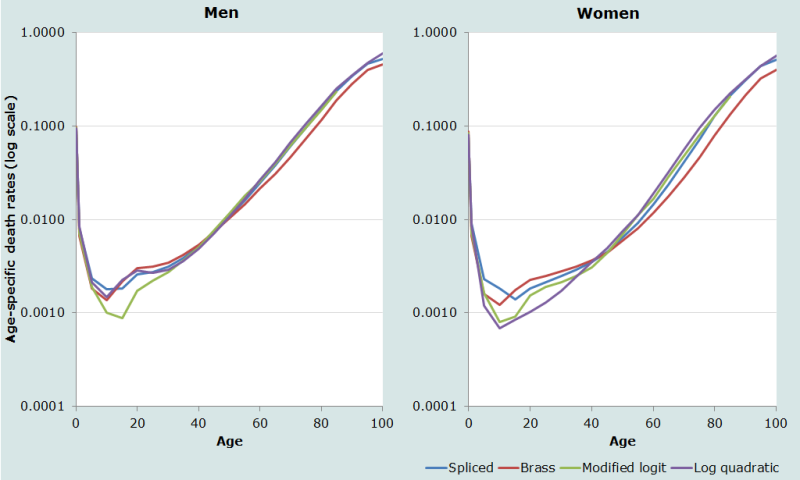
It can be seen from Figure 1 that the death rates in the spliced and log-quadratic models for men are almost identical. The modified logit model also has very similar death rates to these two models in adulthood, but much lower mortality at ages 5-24. The Brass logit model, on the other hand, agrees well with the spliced and log-quadratic models at young ages but has much lower mortality above about age 60 because of the low value of β. The characteristics of the four fitted models for women are similar to those of the models for men except that the log-quadratic model has much lower mortality at ages 10–34 than any of the other models.
Table 4 Indices of mortality in four model life tables fitted to the mortality estimates in Table 3 (West standard life tables)
| Males | Females | |||||||
|---|---|---|---|---|---|---|---|---|---|
| Measure | Splicing | Brass logit | Modified logit | Log quadratic | Splicing | Brass logit | Modified logit | Log quadratic | |
| e0 | 59.7 | 60.9 | 60.3 | 59.3 | 64.3 | 66.6 | 64.4 | 63.9 | |
| 1q0 | 0.0891 | 0.0944 | 0.0923 | 0.0880 | 0.0815 | 0.0842 | 0.0823 | 0.0768 | |
| l(15) | 0.8640 | 0.8679 | 0.8693 | 0.8662 | 0.8737 | 0.8796 | 0.8812 | 0.8836 | |
| 20q60 | 0.6706 | 0.5793 | 0.6771 | 0.7054 | 0.5346 | 0.4050 | 0.5840 | 0.6416 | |
Table 4 illustrates the implications of these differences in the age-specific death rates. The fitted Brass logit models have markedly lower mortality in old age than the other models and appreciably higher life expectancies at birth. On the other hand, the two fitted log-quadratic models have the highest mortality in old age and the lowest life expectancies. The models all yield rather similar estimates of overall survivorship during childhood as a whole (i.e. to age 15). However, the estimates of infant mortality vary materially between the models. Those in the Brass logit models are highest, reflecting the same low values of β that led to low mortality in old age. The substantive implication of these differences between the fitted models is that one cannot hope to estimate either the infant mortality rate or mortality in old age accurately except by measuring them accurately using direct methods.
It should be borne in mind that if the first two models were based on a different standard this would change the characteristics of the fitted life tables relative to the modified logit and log-quadratic models. For example, a Princeton South or UN South Asian standard would produce fitted models using the splicing method and Brass logit system of models that match those from the latter two approaches more closely.
While rather few grounds exist to choose one of the methods over the others, the modified logit and log-quadratic models are theoretically superior to the older approaches to fitting a model life table. Moreover, as outlined in the section on Caveats and Warnings, some empirical evidence exists that suggests that they perform better on average than the splicing method and fitting Brass logit models. Third, in contexts in which it is difficult to determine what standard life table to adopt, this issue can be sidestepped by adopting one of these approaches. Thus, in general, the modified logit and log-quadratic models are to be preferred to the longer-established methods unless evidence exists supporting use of a method based on standards from a particular family of Princeton or United Nations model life tables.
References
Clark SJ. 2019. "A general age-specific mortality model with an example indexed by child mortality or both child and adult mortality," Demography 56(3):1131-1159. doi: https://doi.org/10.1007/s13524-019-00785-3
Murray CJ, BD Ferguson, AD Lopez, M Guillot, J Salomon and O Ahmad. 2003. “Modified logit life table system: principles, empirical validation, and application”, Population Studies 57(2):165–182. doi: https://dx.doi.org/10.1080/0032472032000097083
Preston SH, P Heuveline and M Guillot. 2001. Demography: Measuring and Modelling Population Processes. Oxford: Blackwell.
Wilmoth JR, S Zureick, V Canudas-Romo, M Inoue and C Sawyer. 2012. “A flexible two-dimensional mortality model for use in indirect estimation”, Population Studies 66(1):1–28. doi: https://dx.doi.org/10.1080/00324728.2011.611411
- Printer-friendly version
- Log in to post comments