Indirect estimation from orphanhood in multiple inquiries

Description of the method

The basic orphanhood method estimates the mortality of adult women and men indirectly from data on the survival status of respondents’ mothers and fathers respectively. In order to apply the method, censuses and surveys must minimally have included the questions ‘Is your mother alive?’ and/or ‘Is your father alive?’. By allowing for the mean age at which the mothers and fathers have children in the population concerned, it is possible to convert the proportion of persons in each age group with living mothers and living fathers into life table measures of survivorship in adulthood ($$l_{25+n}/l_{25}$$ for women and $$l_{35+n}/l_{35}$$ for men).

Once data on orphanhood have been collected in two successive inquiries, it is possible to derive synthetic cohort measures of parental survival for the intervening period and estimate life table measures for this period from them. In particular, if adults aged 15 to 49 have been asked about the survival of their parents, one can estimate survivorship from orphanhood in adulthood, which is to say for synthetic cohorts based at age 20. Synthetic cohort methods can provide estimates of adult mortality for a clearly defined and relatively up-to-date period. This is especially useful in countries experiencing generalized HIV epidemics where the level of adult mortality is likely to have changed abruptly in the last couple of decades. The approach also potentially reduces bias resulting from underreporting of orphanhood by respondents who were orphaned at a young age.

If a supplementary question has been asked in a single inquiry about when dead parents died, one can use this information to reconstruct the proportions of respondents with living mothers and fathers at earlier dates and analyze orphanhood in the intervening periods in the same way as data from multiple inquiries.

One advantage that orphanhood methods have over direct questions about deaths in households is that adult mortality can be estimated in this way in moderately-sized inquiries. In contrast, only censuses or unusually large surveys can yield direct estimates based on deaths in the year before the inquiry that are sufficiently precise to be useful. Moreover, orphanhood methods do not assume that the population is closed to migration. However, the results from them will not be representative for small states or sub-national areas in which a substantial proportion of the population are in-migrants or have emigrated.

Data requirements

To estimate the mortality of adult women:

• The proportions of respondents whose mother is alive by five-year age group of respondent at two or more different dates. (Those who did not know or did not declare their mother’s survival status should be excluded from the calculations).
• The number of births in the year before a demographic inquiry tabulated by five-year age group of women giving birth.

To estimate the mortality of adult men:

• The proportion of respondents whose father is alive by five-year age group of respondent at two or more different dates. (Those who did not know or did not declare their father’s survival status should be excluded from the calculations).
• The number of births in the year before a demographic inquiry tabulated by five-year age group of the women giving birth.
• An estimate of the difference between the ages of men and women having children, such as the difference between the median ages of currently married men and women.

These tables should generally be produced separately for male and female respondents and estimates made from both sets of proportions and for the two sexes combined.

The synthetic cohort method described here estimates adult mortality from orphanhood data supplied by adult respondents, which is to say those aged 15 or more years. While no data on younger age groups are required to produce the synthetic cohort estimates, if they were collected they should usually be entered into the spreadsheet so that they can be used to produce estimates by means of the basic orphanhood method.

If sample or design weights have been provided with the data, remember to apply them in the manner appropriate to your statistical software when deriving the tabulations used as inputs.

Important assumptions

An inherent limitation of the orphanhood method is that data on parents’ survival can only be collected from those of their offspring who are alive themselves. The survival of adults who have no living children is unrepresented in the reported proportions of parents alive. Moreover, parents with more than one surviving child are over-represented in comparison to those with exactly one surviving child in proportion to the number of their surviving children. Thus, the method only produces unbiased results if the mortality of parents is unrelated to how many of their children are alive at the time that the data are collected. In general though, the selection bias that arises from breaches in this assumption is small (Palloni, Massagli and Marcotte 1984). In populations affected by generalized HIV epidemics, however, it is likely to be more severe.

Preparatory work and preliminary investigations

Before starting the analysis, one should check how many respondents stated that they did not know whether their mother or, more commonly, father was alive or failed to answer the questions at all. The response rate on these questions is usually very high and one can simply exclude from the analysis those respondents who either answered 'don’t know' or did not answer the question. In effect, this amounts to assuming that the proportion of these respondents’ parents that have died is the same as for respondents that answered the question. However, a few surveys have collected sufficiently incomplete data to suggest that non-response bias could be a substantial problem. For example, it is possible that most people who fail to answer the question have dead parents. If this is the case, such unreported orphans could represent a substantial proportion of all orphans, particularly in the younger age groups, producing a substantial downward bias in the final estimates of mortality.

One useful check on the quality of the orphanhood data is to compare the responses of male and female respondents of the same age. One would not expect the proportion of parents that have died to differ significantly between men and women of the same age. If the proportions diverge among older respondents, this could reflect gender differences in patterns of age misreporting or could indicate that the gender that reports fewer dead parents (usually the men) is more likely to lose touch with their families and is assuming wrongly that some parents remain alive who have died.

When two or more sets of data on the survival of parents are available, one should usually estimate mortality from each set of data independently using the basic orphanhood method as well as produce estimates from synthetic cohort data on orphanhood in adulthood in order to compare the three sets of results. The accompanying Excel workbook produces both basic and synthetic cohort estimates.

Caveats and warnings

• The estimates derived from the orphanhood method are conditional survivorship probabilities, that is to say probabilities of survival across an interval in adulthood conditional on being alive at the start of the interval. To obtain a complete life table, estimates of survivorship from birth to adulthood must be calculated using another source of data on child mortality.
• In a number of applications in East Africa and elsewhere, the orphanhood method has yielded results that indicate implausibly rapid declines in mortality and gross inconsistencies between the estimates from successive enquiries. This appears to be due to ‘the adoption effect’, that is under-reporting of orphanhood among those whose parents die when they are very young (Blacker 1984; Blacker and Gapere 1988; Hill 1984; Timæus 1986). Children who are orphaned at a young age tend to be reared by other relatives and are often enumerated as their own children. This means they are enumerated as having a living parent, and can give rise to very low mortality estimates. Misreporting appears to be particularly common when the mother dies. As the respondents get older, the chance that their foster, adoptive or step-parent has died, as well as their biological parent, increases. This implies that the bias is most pronounced for young children, whose substitute parent is very likely to be alive. Procedures for estimating adult mortality from synthetic cohort data on orphanhood reported by young adults were developed specifically to address this problem, but cannot completely eliminate the bias in the results in populations where orphanhood is severely underreported.
• Although estimates can be made using data on respondents aged in their forties, the parents of many of these respondents are elderly and have very high mortality. This means that the precision with which one can estimate mortality from parental survival data is inherently much lower than it is for younger respondents.
• Like all methods that involve the analysis of change between two independent inquiries, the synthetic cohort approach to the analysis of orphanhood data is vulnerable to bias resulting from differences in data quality between the two inquiries. If respondents were more likely to report dead parents as living in one of the inquiries than the other, the resulting bias will be magnified in the synthetic cohort estimates. Mortality will be overestimated if too few orphans were reported in the earlier inquiry and underestimated if too few orphans were reported in the later inquiry. In addition, estimates based on the change in the proportion of parents that are alive in between two surveys have larger sampling errors than the two sets of proportions from which they are calculated.

Application of method 

Step 1: Calculate the mean ages of childbearing of women and men

To apply the orphanhood method, one requires an estimate of the average age at which the parents had children in order to control for variation in the age range over which they have been exposed to the risk of dying. Women’s mean age of childbearing is usually calculated from census or survey data on births in the last year by five-year age group at interview of the women giving birth. The measure is simply the average age of women giving birth calculated without adjusting for the age structure of the population using the following formula:

$${\overline{M}}^f=\frac{{\displaystyle \sum _{x=15}^{45}{}_{5}B{}_x\left(x+2\right)}}{{\displaystyle \sum _{x=15}^{45}{}_{5}B{}_x}}$$

In this equation, (x + 2) represents the mid-point of the age group of women with a half-year downward shift to allow for the fact that women giving birth in the year before interview did so 6 months ago, on average, and were 6 months younger at that time. This calculation can be done in the accompanying Excel workbook. If the data used to calculate $${\overline{M}}^f$$ are tabulated by women’s age at giving birth, the mid-point of each age group would become x + 2.5.

There is no need to adjust the births data for reference-period errors before calculating $${\overline{M}}^f$$. Moreover, the mortality estimates are not very sensitive to bias in this indicator. However, if evidence exists that the age pattern of births has been distorted severely by women exaggerating their ages, the number of births by age could be recomputed from an adjusted age distribution and adjusted fertility distribution before calculating $${\overline{M}}^f$$.

In principle, the mean age of motherhood should refer to the time at which the respondents were born, which may be any time between 5 and 45 years before the collection of the orphanhood data. An estimate based on fertility data collected in the first of the pair of inquiries that asked about orphanhood should be adequate in populations which at that time had yet to experience substantial fertility decline. If fertility is believed to have fallen and earlier census or survey data exist, $${\overline{M}}^f$$ could also be calculated from the earlier data to determine if it has changed. If it has, then the best way of deciding on final values of $${\overline{M}}^f$$ for the estimation of adult mortality will depend on what data are available and the pattern of change in fertility. One option might be to calculate $${\overline{M}}^f$$ from data collected at about the time that fertility began to fall and use that value for age groups of respondents born then or earlier and to interpolate linearly between that value and the current one to estimate $${\overline{M}}^f$$ for younger age groups of respondents.

The mean age at which men have children is usually estimated by adding an index of the difference in the ages of men and women bearing children to the mean age of childbearing of women:

$${\overline{M}}^m={\overline{M}}^f+d$$

One estimate of this difference that can be readily calculated from census data is the difference between the median ages of currently married men and currently married women. It is more appropriate than the difference between the singulate mean ages at marriage of men and women in populations in which marital dissolution or polygynous marriage is common. The median is used rather than the mean so that differential age exaggeration by older respondents, who are probably no longer bearing children anyway, does not distort the estimate.

This approach to the estimation of the mean age of men at the birth of their children assumes that the ages of the fathers of children born to unmarried women are the same, on average, as the ages of the fathers of children born to married women. They may not be and this could introduce a significant bias into the estimate of $${\overline{M}}^m$$ in populations in which childbearing outside marriage is common. While it is difficult to think of a solution to this problem, fortunately the mortality estimates are not very sensitive to errors in the estimate of $${\overline{M}}^m$$.

Step 2: Calculate the synthetic cohort measures of orphanhood in adulthood

The workbook contains separate sheets for the calculation of these proportions for adult women and for adult men. Either the number of respondents by five-year age group with living mothers and the number answering the question or the proportions with living mothers calculated from them should be entered into the maternal orphanhood sheet. Similarly, either the number of respondents by five-year age group with living fathers and the number answering the question or the proportions with living fathers calculated from them should be entered into the paternal orphanhood sheet. For both the mothers and the fathers, the more recent set of results should be entered in the upper panel of the sheet and the more distant set in the lower panel. While the data can be for female respondents, male respondents, or respondents of both sexes, the two sets of results should usually be tabulated on the same basis.

The spreadsheet calculates the synthetic cohort measures of orphanhood by means of a ‘variable r’ method. The average proportions of respondents with living parents for the period between the two inquiries are multiplied by the exponential of the growth rates in those proportions during the period cumulated from age 20. This ‘removes’ the effect of population growth, producing stationary proportions relative to the proportion with living parents at the base age of 20. These stationary proportions reflect the rate at which adults are being orphaned during the period between the two inquiries.

The average proportion of respondents with living mothers (or fathers) in an age group over the period between the two inquiries is calculated as

$${}_{5}S{}_x(\overline{t})=\sqrt{{}_{5}S{}_x(t)\times {}_{5}S{}_x(t+h)}$$

where t indicates the first inquiry, t + h the second inquiry occurring h years later, and $$\overline{t}$$ a measure applying to the intervening period. Having calculated these measures, the average proportion of the parents of individuals aged exactly 20 that are alive during the period can be estimated as:

$$S(20,\overline{t})=\sqrt{{}_{5}S{}_{15}(\overline{t})\times {}_{5}S{}_{20}(\overline{t})}$$

The growth rates in the proportions of parents that are alive by age group of respondent between the first and second inquiry are calculated as:

$${}_{5}r{}_x(\overline{t})=\frac{\ln ({}_{5}S{}_x(t+h))-\ln ({}_{5}S{}_x(t))}{h}$$

Then the synthetic cohort proportions that have living parents among those who had a living parent at age 20 can be calculated as:

$$\frac{{}_{5}S{}_x(\tau )}{S(20,\overline{t})}=\frac{{}_{5}S{}_x(\overline{t})}{S(20,\overline{t})}\cdot e^{5\left({\displaystyle \sum _{a=20,5}^{x-5}{}_{5}r{}_a(\overline{t})}\right)+2.5{}_{5}r{}_x(\overline{t})}$$

where τ indicates adjusted synthetic cohort (i.e. period) measures for time $$\overline{t}$$.

Step 3a: Calculate the conditional life table survivorship ratios for women

The survivorship of women is estimated between a lower age of 45 and age 25+n, where n is the upper limit of each successive age group of respondents. The following regression equation and the coefficients shown in Table 1 are used:

$${}_{n-20}p{}_{45}=a(n)+b(n){\overline{M}}^f+c(n){}_{5}S{}_{n-5}(\tau )/S(20,\overline{t})$$

For example, when n is 30, life table survivorship is estimated over the ten-year age interval from exact age 45 to exact age 55 using data on survival of mothers supplied by respondents aged 25-29 years.

Table 1 Coefficients for the estimation of women’s survivorship from the proportions of adult respondents with living mothers among those with living mothers at age 20

Step 3b: Calculate the conditional life table survivorship ratios for men

Each estimate of the survivorship of men is produced using data on two adjacent five-year age groups, not a single age group. Men’s survivorship is measured from age 55 to 35 + n, where n is the midpoint of the pair of age groups, using the following regression equation and the coefficients shown in Table 2:

$${}_{n-20}p{}_{55}=a(n)+b(n){\overline{M}}^m+c(n){}_{5}S{}_{n-5}(\tau )/S(20,\overline{t})+d(n){}_{5}S{}_n(\tau )/S(20,\overline{t})$$

For example, when n is 40, life table survivorship is estimated over the 20-year age interval from exact age 55 to exact age 75 using the data on survival of fathers supplied by respondents in the two age groups 35-39 years and 40-44 years.

Table 2 Coefficients for the estimation of men’s survivorship from the proportions of adult respondents with living fathers among those with living fathers at age 20

Step 4: Convert the survivorship ratios into estimates of the level of mortality

The series of conditional survivorship ratios, _np_b, obtained from different age groups of respondents all refer to the interval between the two surveys. They represent incomplete life tables with a base at age 45 for women and age 55 for men. The series will be to some extent erratic as a result of age reporting, sampling, and other errors. It can be smoothed by fitting a 2-parameter logit model life table to the ratios. The logits of the conditional survivorship ratios are calculated as:

$$Y_x=\frac{1}{2}\ln \left(\frac{1-{}_{n}p{}_b}{{}_{n}p{}_b}\right)$$

The equivalent logits of the standard life table are:

$$Y_x^s=\frac{1}{2}\ln \left(\frac{l_b-l_{b+n}}{l_{b+n}}\right)$$

The α and β parameters of the fitted model are the intercept and slope of a regression of the Y_x values on $$Y_x^s$$. In principle, the estimates for older age groups are less vulnerable to sampling error than those on younger age groups as they are based on more parental deaths. However, these estimates can indicate lower mortality than the estimates for younger age groups, perhaps because the respondents are exaggerating their ages. Thus, one should exclude any estimates at either end of the series that are out of line with the others from the range of ages used to estimate α and β.

Once one has calculated α and β, smoothed estimates of conditional survivorship can be calculated as:

$${}_n\widehat{p}{}_b=\frac{1}{1+\exp \left(2\left(\alpha +\beta Y_x^s\right)\right)}$$

The smoothed estimates of conditional survivorship refer to a clearly defined period of time and depend only to a limited extent on assumptions made during the estimation process about the age pattern of mortality. They will not be distorted greatly in populations with unusual age patterns of mortality such as those experiencing generalized HIV epidemics. Thus, if possible, they should be used as they are in further analyses. Nevertheless, it is often necessary to convert the synthetic cohort estimates into a common index of mortality in order to compare those for men and women directly or to compare both series with estimates of mortality from other sources. This can be done by fitting a 1‑parameter model life table to each conditional survivorship ratio and obtaining the desired index from the fitted model.

A wide range of indices have been used for this purpose, including the level parameters of various systems of model life tables, survivorship ratios, life expectancy at various ages between 5 and 30, and temporary life expectancy between ages 25 and 70, ₄₅e₂₅. Using the parameters of the models has the advantage of emphasizing that the full life table is being estimated by fitting a model, rather than measured directly. The measures of life expectancy summarize survivorship across adulthood as a whole, while using survivorship ratios or temporary life expectancies avoids extrapolation into old age from measures for younger adults. Increasingly, in recent years, the estimates have been presented in terms of the probability of dying between exact ages 15 and 60, ₄₅q₁₅, as this measure has found favour with several international agencies as a summary indicator of the mortality of young and middle-aged adults.

In the applications of the orphanhood method presented here the survivorship ratios are converted into the α parameter of a 1-parameter system of logit model life tables, and then into estimates of the conditional probability of dying across a wider range of ages. (Note that, even if the same standard is used and β is 1, the α parameter of a fitted model based at age 0 will not be the same as α in models that have been fitted to measures of conditional survivorship from age 45 or 55.)

The spreadsheet calculates conditional survivorship between exact ages 30 and 60, ₃₀q₃₀, exact ages 15 and 60, ₄₅q₁₅, or exact ages 50 and 70, ₂₀q₅₀. The first two indices are useful for comparing the synthetic cohort estimates with those from the basic orphanhood method and other adult mortality measures respectively; the third is most useful for comparing the estimates made from orphanhood in adulthood for men and women or for assessing the internal consistency of a series of such estimates without extrapolating from survivorship in middle age to younger adult ages. The parameters of the 1-parameter models are calculated from the estimates of _n-20p_b as

$$\alpha =-\frac{1}{2}\ln \left(1+\frac{\frac{{}_{n-20}p{}_b}{l_{b+n-20}^s}-\frac{1}{l_b^s}}{1-{}_{n-20}p{}_b}\right)$$

where the estimates of _n-20p_b come from Step 2, with b = 45 for the estimates of the survivorship of women and b = 55 for those of the survivorship of men, and the $$l_x^s$$values come from a standard life table. Thus, one obtains a series of estimates of α corresponding to the measures of conditional survivorship made from data on the different age groups of respondents. Higher values of α correspond to higher mortality. Then, for each α, summary measures such as ₂₀q­₅₀, ₃₀q₃₀ and ₄₅q₁₅ can be calculated as:

$${}_{n}q{}_b=1-\frac{1+e^{2\left(\alpha +Y_s(b)\right)}}{1+e^{2\left(\alpha +Y_s(b+n)\right)}}$$

The spreadsheet can calculate these measuresusing either a standard from the General set of United Nations model life tables or one from any of the four families of Princeton model life tables. The standard life table should be chosen to have an age pattern of mortality within adulthood that resembles that of the population being studied. Another life tables can be used as a standard instead if there is reason to believe that it resembles more closely the pattern of adult mortality in the population being studied. The most suitable life table may not be from the family of models that best captures the relationship between child and adult mortality. If nothing is known about the age pattern of mortality in adulthood, use of the United Nations General or Princeton West models is recommended.

As the estimates all refer to the same period, it makes sense to produce the final estimate of survivorship for the period between the two inquiries by averaging a contiguous set of estimates that excludes any outlying values made from data on the youngest and oldest respondents. Such outliers can be identified in a plot of the logits of the conditional survivorship ratios against a standard series. If there is a clear upward or downward trend in α across the age groups in the fitted 1-parameter models, the mortality standard to which the estimates are being fitted may be inappropriate. The analysis should probably either adopt another standard or modify the rate at which mortality increases with age in the selected one by adjusting its β parameter.

Step 5: Calculate the time location of the estimates

Each survivorship ratio refers to the period between the dates to which the two sets of orphanhood data refer. One may wish to ascribe them to an exact date within this period, so that they can be plotted and compared with other estimates of adult mortality. If one assumes a constant rate of change in mortality, they can be thought of as referring to the geometric average of the dates of the two inquiries. The date of each inquiry can be calculated as the average of the dates on which the interviews took place or taken as the mid-point of the period of fieldwork if exact dates of interview are not available.

Worked example

This example, implemented in the workbook, uses data on the survival of mothers and fathers collected in the 1989 and 1999 Censuses of Kenya.

Step 1: Calculate the mean ages of childbearing of women and men

For women the mean age of childbearing is a straightforward average of the ages of women giving birth and can either be calculated as such from individual-level data or estimated approximately from a tabulation of births by five-year age group of mother. For this application it has been calculated using data from the first of the pair of censuses (see Table 3), although in Kenya one could also do so using data from previous censuses to check whether ages at childbearing have changed over time:

$${\overline{M}}^f=\frac{16,585,300}{620,000}=26.75$$

Table 3 Calculation of the mean age at childbearing, Kenya, 1989 Census

The mean age of childbearing of men is calculated by adding the difference between the median ages of currently married men and women to the mean age of childbearing of women. It can be seen from Table 4 that the median age of currently married men falls between the mid-point of the age group 30-34 and the mid-point of the age group 35-39. By linear interpolation:

$$\text{Median for men}=32.5+5\times \frac{0.5-0.3886}{0.5272-0.3886}=36.52$$

and

$$\text{Median for women}=27.5+5\times \frac{0.5-0.4234}{0.5597-0.4234}=30.31$$

Table 4 Ages of currently married men and women, Kenya, 1989

Then the estimated mean age of childbearing of men is:

$$M^m=M^f+d=26.75+(36.52-30.31)=32.96$$

Step 2: Calculate the synthetic cohort measures of orphanhood in adulthood

Proportions of Kenyans with living mothers averaged across the period between the 1989 and 1999 censuses of Kenya are shown in the fourth column of Table 5. They are the geometric averages of the proportions reported in the two censuses shown in the second and third columns of the table. For example, in the age group 25-29,

$${}_{5}S{}_{25}(\overline{t})=\sqrt{0.8839\times 0.8771}=0.8805$$

The proportion with living mothers at exact age 20 is calculated from these estimates for age groups 15-19 and 20-24:

$$S(20,\overline{t})=\sqrt{0.9446\times 0.9156}=0.9300$$

Census day in 1999 was 24th August, while in 1989 it was 25th October. Thus, the growth rate over the decade in the proportion of Kenyans with living mothers for the same age group is:

$${}_{5}r{}_{25}(\overline{t})=\frac{\ln (0.8771)-\ln (0.8839)}{9.83}=-0.00078$$

For the first age group, the growth rate cumulated from age 20 to 22.5 is simply:

$$2.5{}_{5}r{}_{20}\left(\overline{t}\right)=-0.00170\times 2.5=-0.00425$$

For the second age group, the growth rate cumulated to age 20 to 27.5 is:

$$5{\displaystyle \sum _{a=20,5}^{20}{}_{5}r{}_a\left(\overline{t}\right)+2.5{}_{5}r{}_{25}\left(\overline{t}\right)}=5\times -0.00170+2.5\times -0.00078=-0.01045$$

while for the third age group it is:

$$5{\displaystyle \sum _{a=20,5}^{25}{}_{5}r{}_a\left(\overline{t}\right)+2.5{}_{5}r{}_{30}\left(\overline{t}\right)}=5\times \left(-0.00170-0.00078\right)+2.5\times 0.00018=-0.01195$$

and so on.

The synthetic cohort proportions that have living mothers among those who had a living mother at age 20 in the seventh column of Table 5 are calculated from the averaged proportions and growth rates in the fourth and fifth columns. For example, for the 25-29 age group,

$$\frac{{}_{5}S{}_x(\tau )}{S(20,\tau )}=\frac{0.8805}{0.9300}\cdot e^{-0.01045}=0.9369$$

The calculations made in this step for the data on paternal orphanhood are identical and are shown in Table 6.

Table 5 Estimation of women’s survivorship in the interval between two inquiries, and corresponding estimates of α and ₃₀q₃₀, from maternal orphanhood in adulthood, Kenya, 1989-99

Step 3a: Calculate the conditional life table survivorship ratios of women

These survivorship ratios are shown in the eighth column of Table 5 and are calculated from the proportions in the seventh column using the regression coefficients shown in Table 1 and the estimate of $${\overline{M}}^f$$ of 26.75 from step 1. For example, for respondents aged 25-29:

$${}_{10}p{}_{45}=-0.3822+0.00679\times 26.75+1.2062\times 0.9369=0.9295$$

Note that each life table measure is similar in value to the proportion from which it was calculated.

Step 3b: Calculate the conditional life table survivorship ratios of men

These survivorship ratios are shown in the eighth column of Table 6 and are calculated from the proportions in the seventh column using the regression coefficients shown in Table 2 and the estimate of $${\overline{M}}^m$$ of 32.96 from Step 1. For example, for the final estimate in Table 6:

$${}_{20}p{}_{55}=-1.1726+0.02647\times 32.96+0.9381\times 0.6156+0.4372\times 0.4772=0.4860$$

Table 6 Estimation of men’s survivorship in the interval between two inquiries, and corresponding estimates of α and ₃₀q₃₀, from paternal orphanhood in adulthood, Kenya, 1989-99

Step 4: Convert the survivorship ratios into estimates of the level of mortality

To smooth the series of estimates of conditional survivorship by fitting a 2-parameter logit model life table to them, one first calculates the logits of the ratios. For example, the estimate of ₁₀p₄₅ for women made from data on respondents aged 25-29 is:

$$Y_x=\frac{1}{2}\ln \left(\frac{1-0.9295}{0.9295}\right)=-1.290$$

The equivalent value for the UN General model life table with e₀=60 is:

$$Y_x^s=\frac{1}{2}\ln \left(\frac{0.7887-0.7103}{0.7103}\right)=-1.102$$

Regressing the logits of the observed estimates of conditional survivorship on the standard logits, excluding the final point (based on respondents aged 45-49) which dips below the line, gives parameter estimates of α = -0.3398 and β =0.8597. The fact that the estimate of β is less than 1 indicates that the mortality of women in Kenya increases less steeply than in the standard across the age range 45 to 75 years.

Having obtained α and β, the smoothed conditional survivorship ratio for the second age group, for example, can be calculated as:

$${}_{10}\widehat{p}{}_{45}=\frac{1}{1+\exp \left(2\left(-0.3398+0.8597\times -1.1016\right)\right)}=\mathrm{0.9291.}$$

The full series of fitted survivorship ratios is shown in the ninth column of Table 5 for women and of Table 6 for men. Taking the estimates of ₅p₄₅ and ₂₅p₄₅ from Table 5, the conditional probability of dying between exact ages 50 and 70 in the fitted 2-parameter model is 1 - 0.7244/0.9667 = 0.251.

Estimates of ₃₀q₃₀, the probability of dying between exact ages 30 and 60, calculated by fitting 1-parameter models to the estimated survivorship ratios, are shown in rightmost columns of Table 5 and Table 6. For example, α is calculated from the estimate of ₁₀p₄₅ for women as:

$$\alpha =-\frac{1}{2}\ln \left(1+\frac{\frac{0.9295}{0.7103}-\frac{1}{0.7887}}{1-0.9295}\right)=-0.228$$

Having calculated α, then the corresponding measure of ₃₀q₃₀ is:

$${}_{30}q{}_{30}=1-\frac{1+e^{2\left(-0.228-0.8655\right)}}{1+e^{2\left(-0.228-0.3064\right)}}=0.172$$

Step 5: Calculate the time location of the estimates

The synthetic cohort estimates are measures of adult mortality during the period between the two inquiries. Their time location can be ascribed to the geometric average of the dates of field work of the two inquiries. Thus, in this application to the 1989 and 1999 Censuses of Kenya:

$$T=\sqrt{1989.81\times 1999.64}=1994.72$$

Diagnostics, analysis and interpretation

Checks and validation

The number of respondents who stated that they did not know whether their mother or father is alive or who did not answer the questions at all should be checked before they are dropped from the analysis. If many of the respondents failed to respond to these questions, the data supplied by those respondents who did answer them may not be representative of the population as a whole. Moreover, a high level of non-response may indicate that either the field staff or the respondents experienced difficulty with the questions. Thus, even when answers were supplied they may be rather unreliable. If a high level of item non-response exists, it can be illuminating to determine whether it is concentrated among a minority of field staff or certain type of respondent.

If information about the survival of mothers and fathers has been collected from both male and female respondents in a census or a large-scale survey with small sampling errors, it is possible to tabulate the proportions of mothers and fathers alive separately for respondents of each sex in order to compare the consistency of their reports. While consistency of reporting does not guarantee accuracy, statistically significant differences between the proportions obtained from male or female respondents imply that at least one sex, and possibly both of them, are answering the questions inaccurately.

It is fairly common to find that women report lower proportions of living parents than men. Some analysts believe that this is because women stay in closer contact with their parents than men and that some men are stating that their parents are alive because they do not know that they have in fact died. If correct, this would imply that the data supplied by women are more accurate. However, no strong evidence exists to support this interpretation and other errors, such as differential age misreporting by male and female respondents, may also produce inconsistencies between the proportions reported by men and women. Because synthetic cohort estimates are calculated, in essence, from the first differences between two sets of proportions, they have larger sampling errors than other orphanhood-based estimates of mortality. Thus, especially if the data come from surveys of a few thousand households, it is advisable to base the final estimates of adult mortality on the combined responses both sexes unless clear evidence exists that one should focus on the data supplied by female respondents.

Interpretation

The results of the example analysis of the orphanhood data from the 1989 and 1999 censuses of Kenya are portrayed graphically in Figure 1. According to the 1989 Census data on orphanhood, adult mortality in Kenya was declining slowly in the late 1970s and early 1980s. The level of mortality was fairly low and a large differential existed between the mortality of men and women. By contrast, the 1999 Census data suggest that mortality rose steadily for both men and women to a considerably higher level between the late-1980s and mid-1990s.

Image

Figure 1 Trends in the conditional probability of dying between exact ages 30 and 60 estimated from orphanhood, Kenya, 1989 and 1999 Censuses

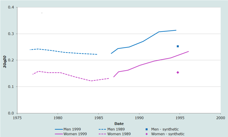
One reassuring feature of these results is that the mortality estimates for 1985-1986 from the two censuses are consistent. Those from the 1989 Census (the most recent points on the dotted lines) are based on reports about the survival of the parents of respondents who are still children. Those for only slightly later made from the 1989 Census (the earliest points on the solid lines) are made from the reports of respondents who were aged in their thirties in 1999. While such consistency between estimates made from the reports of respondents of different ages in different inquiries does not guarantee their accuracy, it is suggestive of it and rules out the presence of certain (but not all possible) errors, including bias resulting from the adoption effect. This effect is most severe for estimates made from data on children because, the younger a child is when its parent dies, the more likely it is that a question about whether the parent is alive will be answered with reference to an adoptive, foster, or step parent who has reared them. As the respondents get older, these misreported cases become proportionately less important compared with the rapidly increasing number of parental deaths that occur as both the respondents and their parents get older. Thus, if the adoption effect was a problem in Kenya one would expect the 1989 Census estimates of adult mortality in the mid-1980s to be lower than the 1999 Census estimates for the same years.

If the mortality estimates obtained from younger respondents by the basic orphanhood method were biased downward, one would expect the synthetic cohort estimates of mortality derived from orphanhood data supplied by young adults to be higher than those from the basic method for the same dates. In Kenya, they are not – they are lower.

This pattern of synthetic data on young adults yielding lower estimates than lifetime data on children is unusual. It probably reflects the growing importance of AIDS mortality in Kenya during the course of the 1990s. The synthetic cohort estimates are based mainly on the experience of parents aged 50 years of more, who have not been affected greatly by the AIDS epidemic. Thus, using standard model life tables to determine ₃₀q₃₀ from these data produces underestimates because mortality at ages 30 to 50 in the fitted models is lower than in Kenya.

In contrast, the parents of the young respondents, whose reports are the basis for the most up-to-date estimates obtained from the basic orphanhood method, are largely in their 30s and 40s. AIDS mortality peaks in this age range. Thus, using standard model life tables to determine ₃₀q₃₀ from these data produces overestimates because mortality at ages 50 to 60 in the fitted models is higher than in Kenya.

The synthetic cohort estimates provide support for this interpretation. In this application, the conditional probability of dying between ages 30 and 60 declines as the age group of the respondents increases for both men and women (see Table 5 and Table 6). This suggests that mortality is relatively high at younger ages within the age range 45 to 75 years and relatively low in late middle age in Kenya compared with United Nations’ General family of model life tables. This is also suggestive of high AIDS mortality among younger adults. The actual value of ₃₀q₃₀ in the mid-1990s probably falls somewhere between the estimates produced by the two variants of the orphanhood method. Adopting a standard age pattern of mortality that increases more slowly with age by setting the β parameter of the standard life table to 0.7 and recalculating α, produces an internally more consistent set of indices for both of the sexes. It also reduces the inconsistencies between the synthetic cohort estimates and the most up-to-date estimates obtained from the 1999 Census data using the basic orphanhood method. Thus, the probability of dying between ages 30 and 60 in Kenya in the mid-1990s, conditional on surviving to age 30, was probably about 20 per cent for women and 30 per cent for men.

Figure 2 presents a second application of the synthetic cohort approach to analyzing two sets of orphanhood data collected in successive inquiries. It analyses data from the 1986 and 1999 Censuses of the Solomon Islands. In this application, the statistic plotted is the probability of dying between ages 15 and 60 conditional on being alive at age 15 (₄₅q₁₅). One immediately obvious contrast between these series of estimates and those for Kenya and the Arab countries for which results are presented in the discussion of the basic orphanhood method is that they suggest that gender inequalities in adult mortality in the Solomon Islands are small.

This application of the estimation method provides clear evidence of problems with the orphanhood data collected in the 1986 Census. First, the estimates suggest that mortality was declining very rapidly but the most recent of the earlier series of estimates, based on data on children, indicate substantially lower mortality than the estimates for a couple of years later that were made using data collected from older respondents in the 1989 Census. Inconsistencies of this sort usually indicate that the more recent estimates from the first of the censuses are too low because orphanhood of children is being underreported due to the adoption effect. Because the tendency to underreport in this way may be an enduring feature of the culture of a population, such inconsistencies also cast doubt on the most recent estimates made from data collected in the later census. The second problem with the estimates from the 1986 Census of the Solomon Islands is that they suggest that women have higher adult mortality than men. This is very uncommon.

Image

Figure 2 Trends in the probability of dying between exact ages 15 and 60 estimated from orphanhood, Solomon Islands, 1986 and 1999 Censuses

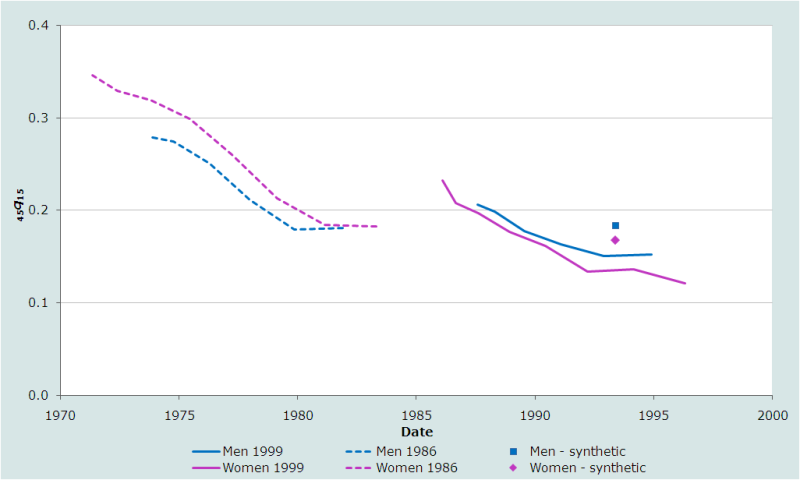
The estimates made for the early 1990s from synthetic cohort data on orphanhood in early adulthood support the suggestion that the lifetime estimates calculated from orphanhood data on children collected in 1999 are also too low. Because they are based exclusively on the reports of adults the synthetic cohort estimates are probably the most reliable estimates presented in Figure 2. Thus, it can be tentatively concluded that the probability of dying between ages 15 and 60 in the Solomon Islands fell from about 30 per cent to about 17.5 per cent in the two decades starting in the early 1970s.

Detailed description of method

Introduction

Simple, robust methods for estimating mortality from cohort data on orphanhood collected in a single inquiry were first published in Brass and Hill (1973). Zlotnik and Hill (1981) were the first to point out that, once the question ‘Is your mother alive?’ or ‘Is your father alive?’ has been asked in two successive inquiries in the same population, it becomes possible to calculate synthetic cohort measures of parental survival from the two sets of answers that reflect adult mortality in the intervening period. Because these estimates are made from changes in parental survival between the two inquiries, they are vulnerable to differential reporting and sampling errors. The time reference of the measures is usually more recent, however, than that of any of the estimates based on respondents' lifetime experience.

Synthetic cohort data also have another advantage: if deaths occurring during the period between the two inquiries are reported fully, omission of more distant deaths will have no impact on the results. Thus, synthetic cohort data on the survival of parents are potentially less vulnerable than lifetime data to the so-called ‘adoption effect’, that is underreporting of orphanhood by respondents whose parents died when the respondents were still young children. This is important because the adoption effect is the major bias affecting the orphanhood method, explaining the implausible results and inconsistencies between successive surveys found in a number of applications of this method.

The most straightforward way of purging the reports of this bias is to analyze only the synthetic cohort data on adults (Timæus 1991). One can do this by constructing a synthetic cohort, based at 20 years of age, from data on parental survival at two dates. This cohort indicates the proportion of the adult population whose mothers or fathers would remain alive, at current levels of mortality, among those who, at exact age 20, had a living mother or father. Such a synthetic cohort can be constructed solely from the relatively reliable data supplied by young adults.

Timæus (1991) proposes basing the cohort at 20 years for two reasons. First, this choice minimizes the possibility of underestimating orphanhood at the base age and consequently overestimating subsequent orphanhood and adult mortality. Second, because information on two age groups is needed to estimate parental survival at the exact age dividing the groups, this approach makes it possible to apply the method to data collected in surveys in which only women aged 15 to 49 are asked about orphanhood.

The generalization to all populations of the relationships between age structure, increase, and mortality stated by stable population theory (Preston and Coale 1982) provides a convenient way of constructing such synthetic cohorts. Stationary synthetic cohort measures of parental survival can be obtained by adjusting the reported proportions with living parents using the age-specific growth rates in these proportions to remove the impact of past trends in mortality. When the data come from two inquiries, adjustment using age-specific rates of increase in parental survival has the advantage over methods based on chaining cohort changes of being easy to apply to an interval between the inquiries of other than five and ten years.

Mathematical exposition

Preston and Coale (1982) show that in any closed population defined by age:

$$N(0,t)=N(a,t)\cdot e^{{\displaystyle \underset{0}{\overset{a}{\int }}\mu (z,t)dz}}\cdot e^{{\displaystyle \underset{0}{\overset{a}{\int }}r(z,t)dz}}$$

where N(a,t) is the number of individuals aged a at time t and μ(z,t) and r(z,t) are the force of mortality and rate of growth respectively at age z and time t. Attrition of the population with living mothers or living fathers, denoted NO, can be decomposed into the mortality of the parents and the mortality of the population itself (Preston and Chen 1984; Timæus 1986):

$$NO(0,t)=NO(a,t)\cdot e^{{\displaystyle \underset{0}{\overset{a}{\int }}\mu (z,t)dz}}\cdot e^{{\displaystyle \underset{0}{\overset{a}{\int }}\pi (z,t)dz}}\cdot e^{{\displaystyle \underset{0}{\overset{a}{\int }}{r}^{NO}(z,t)dz}}$$

where π(z,t) represents the instantaneous rate of orphanhood, and r^NO(z,t) the rate of growth of the population with living parents, at age z and time t. Assuming that orphans and the rest of the population have identical mortality and using the fact that N(0,t) ≡ NO(0,t), division of the expression for non-orphans by that for the total population produces

$$e^{-{\displaystyle \underset{0}{\overset{a}{\int }}\pi (z,t)dz}}=\frac{NO(a,t)}{N(a,t)}\cdot e^{{\displaystyle \underset{0}{\overset{a}{\int }}{r}^{NO}(z,t)-r(z,t)dz}}$$

Taken as a whole, the left-hand term represents the stationary probability of an individual aged a having a living mother or father, denoted S(a,τ), whereas NO(a,t)/N(a,t) equals the equivalent unadjusted proportion, S(a,t). With survey data, it is more convenient to work with the rate of increase in the proportion of the population with living parents, r^s(z,t), than with its equivalent, r^NO(z,t) - r(z,t), the difference between the rates of increase for the non-orphaned and the total populations.

The population above any given age can be treated as self-contained and the relationship between age structure, increase, and mortality stated in Equation 1 will continue to hold for such populations. Thus, using the notation already established:

$$\frac{NO(20,t)}{N(20,t)}{e}^{-{\displaystyle \underset{20}{\overset{a}{\int }}\pi (z,t)dz}}=\frac{NO(a,t)}{N(a,t)}\cdot e^{{\displaystyle \underset{20}{\overset{a}{\int }}{r}^s(z,t)dz}}$$

for a > 20. When both sides are divided by S(20, t) this becomes:

$$\frac{S(a,\tau )}{S(20,\tau )}=\frac{S(a,t)}{S(20,t)}\cdot e^{{\displaystyle \underset{20}{\overset{a}{\int }}{r}^s(z,t)dz}}$$

In discrete form, for age groups x to x+5:

$$\frac{{}_{5}S{}_x(\tau )}{S(20,\tau )}=\frac{{}_{5}S{}_x(t)}{S(20,t)}\cdot e^{5\left({\displaystyle \sum _{z=20,5}^{x-5}{}_{5}r{}_z}(t)\right)+2.5{}_{5}r{}_x(t)}$$

Implementation of the method

In order to simplify the estimation of life table measures of mortality from these proportions, Timæus (1991) developed regression models for both men’s and women’s mortality estimating the coefficients from data on parental survival in the same set of simulated populations used to estimate those for the basic orphanhood method (Timæus 1992).

The proportion of individuals aged a that have living mothers, S(a), can be calculated as the average of the probabilities of surviving among mothers who gave birth at each age y, weighting by the proportion of births that occur at y (Brass and Hill 1973):

$$S(a)=\frac{{\displaystyle \underset{s}{\overset{\omega }{\int }}{e}^{-ry}f(y)l(y+a)dy}da}{{\displaystyle \underset{s}{\overset{\omega }{\int }}{e}^{-ry}f(y)l(y)dy}}$$

where integration is over all ages at child bearing s to ω. Dividing S(a) by S(20) for a > 20, the denominators cancel. Thus, the proportion of a five-year age group with living mothers among those who had a living mother at exact age 20 is:

$$\frac{{}_{5}S{}_x}{S(20)}=\frac{{\displaystyle \underset{x}{\overset{x+5}{\int }}{e}^{-ra}l(a){\displaystyle \underset{s}{\overset{\omega }{\int }}{e}^{-ry}f(y)l(y+a)dy}da}}{{\displaystyle \underset{x}{\overset{x+5}{\int }}{e}^{-ra}l(a)da{\displaystyle \underset{s}{\overset{\omega }{\int }}{e}^{-ry}f(y)l(y+20)dy}}}$$

for x≥20. The equivalent proportion in each age group with living fathers is:

$$\frac{{}_{5}S{}_x}{S(20)}=\frac{{\displaystyle \underset{x}{\overset{x+5}{\int }}{e}^{-ra}l(a){\displaystyle \underset{s}{\overset{\omega }{\int }}{e}^{-ry}f(y)l(y)l(y+a)/l(y-0.75)dy}da}}{{\displaystyle \underset{x}{\overset{x+5}{\int }}{e}^{-ra}l(a)da{\displaystyle \underset{s}{\overset{\omega }{\int }}{e}^{-ry}f(y)l(y)l(y+20)/l(y-0.75)dy}}}$$

where f(y) represents the age-specific fertility schedule, and l(a) the life table survivorship, of men rather than of women and the ages between which childbearing occurs s and ω are also those of men.

Equations 3 and 4 can be evaluated numerically using model life tables and fertility schedules and different age structures. Then a regression model that predicts life table survivorship can be fitted to these simulated data on parental survival. The estimation equation used for maternal orphanhood after age 20 is analogous to those proposed for orphanhood since birth (Timæus 1991, 1992). It is based on the observation that the proportion of respondents with living mothers equals a life table survivorship ratio, $$l(B+N)/l(B)$$, where N is the age of the respondents and B lies close to the mean age at childbearing, but also depends on N (Brass and Hill 1973). For practical applications, however, it is more convenient to adjust the proportions slightly on the basis of the mean age at childbearing and to estimate survivorship for a rounded base age, b, close to B, and a duration of exposure, n, which is a multiple of five years. Moreover, for orphanhood after age 20 years, exposure starts 20 years after B. Thus, survivorship is estimated from a base age of 45 years and the equation used to make the estimates takes the form:

$${}_{n-20}p{}_{45}=a(n)+b(n){\overline{M}}^f+c(n){}_{5}S{}_{n-5}(\tau )/S(20,\overline{t})$$

The equivalent equation sometimes gives poor results for men. More accurate estimates can be obtained if information on the survival of fathers in two adjoining age groups is used to infer mortality. If age patterns of mortality and childbearing differ from the average patterns reflected in the regression coefficients, the proportions of respondents with a living father in the upper age group and in the lower age group are shifted in compensating directions in comparison to the proportion at the age dividing the two groups (Timæus 1992). If one estimates life table measures from data on two age groups for a duration of exposure equal to their midpoint, one reduces the sensitivity of the results to variation in the slope of the relationship between parental survival and life table survivorship. The mean age of childbearing of men in developing countries averages a little less than 35 years. Thus, survivorship ratios can be estimated from orphanhood after age 20 by using a base age of 55 years and a model of the form:

$${}_{n-20}p{}_{55}=a(n)+b(n){\overline{M}}^m+c(n){}_{5}S{}_{n-5}(\tau )/S(20,\overline{t})+d(n){}_{5}S{}_n(\tau )/S(20,\overline{t})$$

The coefficients for the different age groups defined by n are presented in Table 1 and Table 2.

Extensions of the method

Chackiel and Orellana (1985) point out that, in addition to analyzing orphanhood data from two inquiries using methods for synthetic cohorts, one can collect data in a single inquiry that can be used to produce up-to-date estimates in the same way. What is required in addition to the usual items about parental survival is information on the dates when parents died. For example, the inquiry might ask about the year and month when the parent died or how many years ago they died. If the dates when parents died are reported with reasonable accuracy, this information can be used to reconstruct the proportion of respondents who had living parents five and ten years earlier. From these successive cross-sections, one can construct synthetic cohort measures of parental survival that are formally identical to those generated from data collected in a series of separate inquiries. Thus, they can be analyzed using the procedure for estimating mortality from orphanhood in adulthood that is described here with reference to data from multiple inquiries.

Rather few inquiries have tried to collect information on when parents died. In some of them the quality of the responses has been very poor, but in other inquiries the reported dates of occurrence of deaths in the previous decade or so, which are the deaths that are of most analytic interest, seem to have been quite well reported.

An alternative way of distinguishing between more recent and more distant death of parents that may yield better quality data is to ask whether parents died before or after some other important demographic event in the respondents’ past, such as getting married or becoming a parent. Methods for making estimates of mortality from data of this type are described alongside other methods for the analysis of orphanhood data from a single inquiry.

Further reading and references

The basic orphanhood method is discussed in all the classic manuals on indirect estimation (Sloggett, Brass, Eldridge et al. 1994; UN Population Division 1983) but, with the exception of the United Nations manual on estimating adult mortality (UN Population Division 2002), these manuals give emphasis to the older variant of the method that uses weighting factors to produce life table indices, rather than the regression-based method normally used today. Although regression-based methods for women had been proposed previously (Hill and Trussell 1977; Palloni and Heligman 1985), regression methods for estimating men’s mortality were first developed by Timæus (1992). His article also surveys earlier contributions to the literature and discusses the theoretical basis of the method.

Methods for constructing parental survival data for synthetic cohorts and estimating adult mortality from them were first proposed in the 1980s (Chackiel and Orellana 1985; Timæus 1986; UN Population Division 1983; Zlotnik and Hill 1981). The version of this approach that focuses on orphanhood after age 20 and is described here was first proposed by Timæus (1991).

Blacker JGC. 1984. "Experiences in the use of special mortality questions in multi-purpose surveys: the single-round approach," in Data Bases for Mortality Measurement. New York: United Nations, pp. 79-89. https://www.un.org/development/desa/pd/sites/www.un.org.development.desa.pd/files/publications/mortality/mortality_1984_databasesformortalitymeasurements.pdf

Blacker JGC and JM Gapere. 1988. “The indirect measurement of adult mortality in Africa: results and prospects,” in African Population Conference, Dakar, 1988. Liège: International Union for the Scientific Study of Population, Vol. 2:3.2.23–38.

Brass W and K Hill. 1973. “Estimating adult mortality from orphanhood,” in International Population Conference, Liège, 1973. Liège: International Union for the Scientific Study of Population,  Vol. 3:111–123.

Chackiel J and H Orellana. 1985. “Adult female mortality trends from retrospective questions about maternal orphanhood included in censuses and surveys,” in International Population Conference, Florence, 1985. Liège: International Union for the Scientific Study of Population, Vol. 4:39–51.

Hill K. 1984. "An evaluation of indirect methods for estimating mortality," in Vallin, J, Pollard John H and L Heligman (eds). Methodologies for the Collection and Analysis of Mortality Data. Liège: Ordina, pp. 145-176.

Hill K and TJ Trussell. 1977. "Further developments in indirect mortality estimation", Population Studies 31(2):313-334. doi: https://dx.doi.org/10.1080/00324728.1977.10410432

Palloni A and L Heligman. 1985. "Re-estimation of structural parameters to obtain estimates of mortality in developing countries", Population Bulletin of The United Nations 18:10-33. https://www.un.org/development/desa/pd/sites/www.un.org.development.desa.pd/files/files/documents/2020/Jan/un_1986_population_bulletin_18.pdf

Palloni A, M Massagli and J Marcotte. 1984. "Estimating adult mortality with maternal orphanhood data: analysis of sensitivity of the techniques", Population Studies 38(2):255-279. doi: https://dx.doi.org/10.1080/00324728.1984.10410289

Preston SH and N Chen. 1984. Two Census Orphanhood Methods for Estimating Adult Mortality, with Applications to Latin America..

Preston SH and AJ Coale. 1982. "Age structure, growth, attrition and accession: A new synthesis", Population Index 48(2):217-259.

Sloggett A, W Brass, SM Eldridge, IM Timæus, P Ward and B Zaba. 1994. Estimation of Demographic Parameters from Census Data. Tokyo, Japan: United Nations Statistical Institute for Asia and the Pacific.

Timæus I. 1986. "An assessment of methods for estimating adult mortality from two sets of data on maternal orphanhood", Demography 23(3):435-450. doi: https://dx.doi.org/10.2307/2061440

Timæus IM. 1991. "Estimation of mortality from orphanhood in adulthood", Demography 28(2):213-227. doi: https://dx.doi.org/10.2307/2061276

Timæus IM. 1992. "Estimation of adult mortality from paternal orphanhood: a reassessment and a new approach", Population Bulletin of The United Nations 33:47-63. https://www.un.org/development/desa/pd/sites/www.un.org.development.desa.pd/files/files/documents/2020/Jan/un_1992_population_bulletin_33.pdf

UN Population Division. 1983. Manual X: Indirect Techniques for Demographic Estimation. New York: United Nations, Department of Economic and Social Affairs, ST/ESA/SER.A/81. https://www.un.org/development/desa/pd/sites/www.un.org.development.desa.pd/files/files/documents/2020/Jan/un_1983_manual_x_-_indirect_techniques_for_demographic_estimation.pdf

UN Population Division. 2002. Methods for Estimating Adult Mortality. New York: United Nations, Department of Economic and Social Affairs, ESA/P/WP.175. https://www.un.org/development/desa/pd/sites/www.un.org.development.desa.pd/files/files/documents/2020/Jan/un_2002_methodsestimatingadultmort.pdf

Zlotnik H and KH Hill. 1981. "The use of hypothetical cohorts in estimating demographic parameters under conditions of changing fertility and mortality", Demography 18(1):103-122. doi: https://dx.doi.org/10.2307/2061052