Indirect estimation of adult mortality from orphanhood

Description of the method

Orphanhood methods estimate the mortality of adult women and men indirectly from data on the survival status of respondents’ mothers and fathers respectively. In order to apply the method, at least one census or single-round survey of the population must have included the questions ‘Is your mother alive?’ and ‘Is your father alive?’. Mortality can be estimated from the answers to these questions without requiring respondents to recall the dates when deaths occurred or the ages at death of deceased individuals.

Since respondents’ mothers must have been alive when the respondents were born, the duration over which they have been exposed to the risk of dying equals the age of the respondents. By allowing for the mean age at which the mothers gave birth in the population concerned, it is possible to predict life table survivorship from age 25 to age 25 plus a rounded number of years (n) based on the age group of the respondents ($$l_{25+n}/l_{25}$$) from the proportion of respondents in each age group whose mother is alive. Similarly, by adjusting for the mean age at which the fathers have children, one can predict life table survivorship of adult men from the proportions of respondents with living fathers. As men tend to be older than their wives and other partners, their survivorship is measured between a base age of 35 and age 35+n where n is again linked to the age group of the respondents.

If mortality has changed over time, the estimated survivorship ratios reflect the mortality rates that have prevailed at a range of ages and dates. A ‘time location’ method has been developed that estimates how many years prior to inquiry each cohort survivorship ratio equalled the period survivorship ratio. These intervals increase with the age of respondents, ranging between about 4 and 14 years before the collection of the data. Thus, if the survivorship ratios estimated from the reports of different age groups of respondent are translated into a common index of mortality in adulthood (such as ₄₅q₁₅) using a 1-parameter system of model life tables, these statistics will refer to different dates and can be used to infer the broad trend in mortality over time.

One advantage that orphanhood methods have over questions about household deaths is that only censuses or unusually large surveys can capture information on enough deaths in households in the year before the inquiry to yield mortality estimates that are sufficiently precise to be useful. The orphanhood method can be used in much smaller inquiries, although all methods for the estimation of adult mortality require data on thousands of households. Moreover, the method does not assume that the population is closed to migration. However, the results from the method will not be representative for small states or sub-national areas in which a substantial proportion of the population are in-migrants or have emigrated.

Data requirements and assumptions

Tabulations of data required

To estimate the mortality of adult women:

• The proportion of respondents whose mother is alive by five-year age group of respondent. (Those who did not know or did not declare their mother’s survival status should be excluded from the calculations.)
• The number of births in the year before a demographic inquiry tabulated by five-year age group of the women giving birth.

To estimate the mortality of adult men:

• The proportion of respondents whose father is alive by five-year age group of respondent. (Those who did not know or did not declare their father’s survival status should be excluded from the calculations.)
• The number of births in the year before a demographic inquiry tabulated by five-year age group of the women giving birth.
• An estimate of the difference between the ages of men and women having children, such as the difference between the median ages of currently married men and women.

These tables should generally be produced separately for male and female respondents and estimates made from both sets of proportions and for the two sexes combined.

For the purposes of estimating mortality, ideally everyone aged less than 50 should be asked the questions about the survival of their mothers and fathers (it may be simpler just to ask everyone these questions). Nevertheless, if an inquiry only asked about the orphanhood of children, the data can be used to produce point estimates of women’s and men’s mortality a few years earlier.

If sample or design weights have been provided with the data, remember to apply them in the manner appropriate to your statistical software when deriving the tabulations used as inputs.

Important assumptions

An inherent limitation of the orphanhood method is that data on parents’ survival can only be collected from those of their offspring who are alive themselves. The survival of adults who have no living children is unrepresented in the reported proportions of parents alive. Moreover, parents with more than one surviving child are over-represented in comparison to those with exactly one surviving child in proportion to the number of their surviving children. Thus, the method only produces unbiased results if the mortality of the parents is unrelated to how many of their children are alive at the time that the data are collected. In general, the selection bias that arises from breaches in this assumption is small (Palloni, Massagli and Marcotte 1984). In populations affected by generalized HIV epidemics, however, it is likely to be more severe. Methods that at least partially address the specific biases that exist in such populations are discussed in a separate section of this webpage on orphanhood in populations affected by AIDS.

The method estimates the trend in mortality from data supplied by different age groups of respondent: the older the respondent, the longer ago their parents died on average. In order to convert the series of measures of survivorship obtained from different age groups into a single indicator that can be compared over time, it must be assumed that the age pattern of mortality in adulthood is represented by the chosen standard life table. To estimate the time location of these measures, it is further assumed that mortality declined linearly in terms of that standard over the period being considered. Both assumptions are likely to be problematic in populations experiencing generalized HIV epidemics

Preparatory work and preliminary investigations

Before starting the analysis, one should check how many respondents stated that they did not know whether their mother or, more commonly, father was alive or failed to answer the questions at all. The response rate on these questions is usually very high and one can simply exclude from the analysis those respondents who either answered 'don’t know' or did not answer the question. In effect, this amounts to assuming that the proportion of these respondents’ parents that have died is the same as for respondents that answered the question. However, a few surveys have collected sufficiently incomplete data to suggest that non-response bias could be a substantial problem. For example, it is possible that most people who fail to answer the question have dead parents. If this is the case, such unreported orphans could represent a substantial proportion of all orphans, particularly in the younger age groups, producing a substantial downward bias in the final estimates of mortality.

One useful check on the quality of the orphanhood data is to compare the responses of male and female respondents of the same age. One would not expect the proportion of parents that have died to differ significantly between men and women of the same age. If the proportions diverge among older respondents, this could reflect gender differences in patterns of age misreporting or could indicate that the gender that reports fewer dead parents (usually the men) is more likely to lose touch with their families and is assuming wrongly that some parents remain alive who have died.

Caveats and warnings

• The estimates derived from the orphanhood method are conditional survivorship probabilities, that is to say probabilities of surviving across an interval in adulthood conditional on being alive at the start of the interval. To obtain a complete life table, estimates of survivorship from birth to adulthood must be calculated using another source of data on child mortality.
• Deaths of parents do not occur at one point in time but may have occurred at any time between the respondents’ birth and when they were interviewed. Thus, the orphanhood method can only indicate the smoothed trend in adult mortality and will fail to capture short-term mortality crises or abrupt reversals in the trend in mortality such as those resulting from AIDS after the onset of a generalized HIV epidemic.
• The most up-to-date mortality estimates that can be produced using orphanhood data are made from those on children aged 5 to 14. Typically only a few per cent of children are maternal orphans and the resulting estimates can have wide confidence intervals even in large sample surveys.
• In a number of applications in East Africa and elsewhere, the orphanhood method has yielded results that indicate implausibly rapid declines in mortality and gross inconsistencies between the estimates from successive enquiries. This appears to be due to ‘the adoption effect’, that is under-reporting of orphanhood among those whose parents die when they are very young (Blacker 1984; Blacker and Gapere 1988; Hill 1984; Timæus 1986). Children who are orphaned at a young age tend to be reared by other relatives and are often enumerated as their own children. This means they are enumerated as having a living parent and can give rise to very low mortality estimates. Misreporting appears to be particularly common when the mother dies. As the respondents get older, the chance that their foster, adoptive or step-parent has died, as well as their biological parent, increases. This implies that the bias is most pronounced for young children, whose substitute parent is very likely to be alive. Thus, if it is not recognized, the adoption effect leads to the underestimation of recent adult mortality and an overestimate of the extent of mortality decline.
• Although estimates can be made using data on respondents aged in their forties, the parents of many of these respondents are elderly and have very high mortality. This means that the precision with which one can estimate both mortality from parental survival data and the reference dates of the estimates is inherently much lower than it is for younger respondents.
• The orphanhood method does not involve the assumption that the population is closed to migration. Nevertheless, it can be difficult to interpret orphanhood-based estimates of adult mortality for sub-national geographic units, such as urban and rural areas or districts, or for respondents with particular socio-economic characteristics. Some or many of the respondents’ parents will live in different places from the respondents themselves and their socio-economic characteristics may differ from those of their children. However, parents and children usually do share the same ethnic identity.

Application of method

Maternal orphanhood

Step 1a: Calculate the mean age of childbearing of women, $${\overline{M}}^f$$

To apply the orphanhood method, one requires an estimate of the average age at which the parents had their children in order to control for variation in the age range over which they have been exposed to the risk of dying. Women’s mean age of childbearing is usually calculated from census or survey data on recent births by five-year age group at interview of the women giving birth. The measure is simply the average age of women giving birth calculated without adjusting for the age structure of the population using the following formula:

$${\overline{M}}^f=\frac{{\displaystyle \sum _{x=15}^{45}{}_{5}B{}_x\left(x+2\right)}}{{\displaystyle \sum _{x=15}^{45}{}_{5}B{}_x}}$$

In this equation, ₅B_x represents births to women in the age group x to x + 4 completed years and (x + 2) represents the mid-point of the age group of women with a half-year downward shift to allow for the fact that women giving birth in the year before interview did so 6 months ago, on average, and were 6 months younger at that time. This calculation can be done in the accompanying Excel workbook. If the data used to calculate $${\overline{M}}^f$$ are tabulated by women’s age at giving birth, the mid-point of each age group would become x+2.5.

There is no need to adjust the births data for reference-period errors before calculating $${\overline{M}}^f$$. Moreover, the mortality estimates are not very sensitive to bias in this indicator. However, if evidence exists that the age pattern of births has been distorted severely by women exaggerating their ages, the number of births by age could be recomputed from an adjusted age distribution and adjusted fertility distribution before calculating $${\overline{M}}^f$$.

In principle, the mean age of motherhood should refer to the time at which the respondents were born, which may be any time between 5 and 45 years before the collection of the orphanhood data. An estimate based on fertility data collected in the same enquiry that asked about orphanhood should be indequate in populations which have yet to experience substantial fertility decline. If fertility is believed to have fallen and earlier census or survey data exist, $${\overline{M}}^f$$ could also be calculated from the earlier data to determine if it has changed. If it has, then the best way of deciding on final values of $${\overline{M}}^f$$ for the estimation of adult mortality will depend on what data are available and the pattern of change in fertility. One option might be to calculate $${\overline{M}}^f$$ from data collected at about the time that fertility began to fall and use that value for age groups of respondents born then or earlier and to interpolate linearly between that value and the current one to estimatefor younger age groups of respondents.

Step 2a: Calculate the conditional life table survivorship ratios for women

The accompanying Excel workbook contains separate sheets for the calculation of the survivorship ratios for adult women (maternal orphanhood) and adult men (paternal orphanhood). The sheets are set up both to analyse data on male and female respondents separately and to combine them to produce estimates based on the data supplied by both sexes. Either the number of respondents of each sex by five-year age group with living mothers and number answering the question or the proportions with living mothers calculated from them should be entered into the maternal orphanhood sheet. Data on respondents aged 5 to 49 years can be used.

Women’s survivorship is estimated between a lower age of 25 and age 25 + n, where n is the upper limit of each successive age group of respondents. The following regression equation and the coefficients shown in Table 1 are used:

$${}_{n}p{}_{25}=a(n)+b(n){\overline{M}}^f+c(n){}_{5}S{}_{n-5}$$

where ₅S_n-5 is the proportion of respondents in the age group from exact age n-5 to exact age n with living mothers. For example, when n is 10, life table survivorship is estimated over the 10-year age interval from exact age 25 to exact age 35 using data on survival of mothers supplied by respondents aged 5-9 years.

Table 1 Coefficients for the estimation of women’s survivorship from the proportions of respondents with living mothers 

n	a(n)	b(n)	c(n)
10	-0.2894	0.00125	1.2559
15	-0.1718	0.00222	1.1123
20	-0.1513	0.00372	1.0525
25	-0.1808	0.00586	1.0267
30	-0.2511	0.00885	1.0219
35	-0.3644	0.01287	1.0380
40	-0.5181	0.01795	1.0753
45	-0.6880	0.02343	1.1276
50	-0.8054	0.02721	1.1678
Source: Timæus (1992)

 

Paternal orphanhood

Step 1b: Calculate$${\overline{M}}^m$$, the mean age of childbearing of men

In principle, the best way to calculate the mean age at which men have children is to calculate the mean age of the partners of women who gave birth in a defined year. However, this method requires data on women to be linked to those on their partners, which is impossible in many datasets.

Thus, the mean age at which men have children is usually estimated by adding an index of the difference between the ages of men and women who are having children to the mean age of childbearing of women:

$${\overline{M}}^m={\overline{M}}^f+d$$.

One estimate of this difference that can be readily calculated from census data is the difference between the median ages of currently married men and currently married women. It is more appropriate than the difference between the singulate mean ages at marriage of men and women in populations in which marital dissolution or polygynous marriage is common. The median is used rather than the mean so that differential age exaggeration by older respondents, who are probably no longer bearing children anyway, does not distort the estimate.

This approach to the estimation of the mean age of men at the birth of their children assumes that the ages of the fathers of children born to unmarried women are the same, on average, as the ages of the fathers of children born to married women. They may not be and this could introduce a significant bias into the estimate of $${\overline{M}}^m$$ in populations in which childbearing outside marriage is common. While it is difficult to think of a solution to this problem, fortunately the mortality estimates are not very sensitive to errors in the estimate of $${\overline{M}}^m$$.

Step 2b: Calculate the conditional life table survivorship ratios for men

The accompanying Excel workbook contains separate sheets for the calculation of the survivorship ratios for adult women and adult men. Either the number of respondents by five-year age group with living fathers and number answering the question or the proportions with living fathers calculated from them should be entered into the paternal orphanhood sheet. Data are used only on respondents aged 5 to 44 years.

Each estimate of men’s survivorship is produced using data on two adjacent five-year age groups. For every pair of age groups except the youngest pair analysed, men’s survivorship is measured from age 35 to 35+n, where n is the midpoint of the pair of age groups using the following regression equation and the coefficients shown in Table 2:

$${}_{n}p{}_{35}=a(n)+b(n){\overline{M}}^m+c(n){}_{5}S{}_{n-5}+d(n){}_{5}S{}_n$$

For example, when n is 10, life table survivorship is estimated over the 10-year age interval from exact age 35 to exact age 45 using the data on survival of fathers supplied by respondents in the two age groups 5-9 years and 10-14 years.

For the youngest pair of age groups, however, this survivorship ratio is much higher than the proportions of fathers alive, which makes the estimates very sensitive to the exact age pattern of mortality in the population. More robust estimates are obtained using the equation:

$${}_{15}p{}_{35}=a(10)+b(10){\overline{M}}^m+c(10){}_{5}S{}_5+d(n){}_{5}S{}_{10}$$

In other words, the same survivorship ratio, ₁₅q₃₅, is estimated from data on respondents aged both 5-14 and 10-19.

Table 2 Coefficients for the estimation of men’s survivorship from the proportions of respondents with living fathers

n	a(n)	b(n)	c(n)	d(n)
10	-0.5578	0.00040	1.4708	0.0698
15	-0.4013	0.00576	1.5602	-0.3522
20	-0.3329	0.01031	0.6656	0.3419
25	-0.4726	0.01559	0.2161	0.7896
30	-0.7056	0.02076	0.1997	0.9066
35	-0.9153	0.02493	0.3484	0.8631
40	-0.9950	0.02635	0.4269	0.8263
Source: Timæus (1992)

Maternal and paternal orphanhood

Step 3: Convert the survivorship ratios into estimates of the level of mortality

To infer mortality trends from a series of survival ratios, _np_b, obtained from different age groups of respondents and referring to different dates, it is necessary to convert them all into a common index of mortality that can be compared over time. This is done by fitting a 1‑parameter model life table to each measure and obtaining the common mortality index from the model.

A wide range of indices have been used for this purpose, including the level parameters of various systems of model life tables, survivorship ratios such as ₃₅p₃₀, which correspond fairly closely to the age range of the estimates yielded by the orphanhood method, life expectancy at various ages between 5 and 30, and temporary life expectancy between ages 25 and 70, ₄₅e₂₅. Using the parameters of the models has the advantage of emphasizing that the full life table is being estimated by fitting a model, rather than measured directly. The measures of life expectancy summarize survivorship across adulthood as a whole, while using survivorship ratios or temporary life expectancies avoids extrapolation into old age from measures for younger adults. Increasingly, in recent years, the estimates have been presented in terms of the probability of dying between exact ages 15 and 60, ₄₅q₁₅, as this measure has found favour with several international agencies as a summary indicator of the mortality of young and middle-aged adults.

In the applications of the orphanhood method presented here the survivorship ratios are converted into the α parameter of a 1-parameter system of relational logit model life tables, and then into either estimates of the probability of dying between exact ages 15 and 60, ₄₅q₁₅, or the probability of dying between exact ages 30 and 60, ₃₀q₃₀. The latter measure is useful for comparing series of orphanhood estimates with each other without extrapolating from mortality across one age range to mortality across another by more than is necessary. The parameters of the 1-parameter models are calculated from the estimates of _np_b as:

$$\alpha =-\frac{1}{2}\ln \left(1+\frac{\frac{{}_{n}p{}_b}{l_{b+n}^s}-\frac{1}{l_b^s}}{1-{}_{n}p{}_b}\right)$$

where the estimates of _np_b come from Step 2 with b = 25 for the estimates of women’s survivorship and b = 35 for those of men’s survivorship and the $$l_x^s$$ values come from a standard life table. Thus, one obtains a series of values of α corresponding to the measures of conditional survivorship made from data on the different age groups of respondents. Higher values of α correspond to higher mortality. Then, for each α:

$${}_{45}q{}_{15}=1-\frac{1+e^{2\left(\alpha +Y_s(15)\right)}}{1+e^{2\left(\alpha +Y_s(60)\right)}}$$

or

$${}_{30}q{}_{30}=1-\frac{1+e^{2\left(\alpha +Y_s(30)\right)}}{1+e^{2\left(\alpha +Y_s(60)\right)}}$$

The accompanying spreadsheet can calculate α, ₄₅q₁₅, and ₃₀q₃₀ using either a standard from the General family of United Nations model life tables or one from any of the four families of Princeton model life tables. The standard life table should be chosen to have an age pattern of mortality within adulthood that resembles that of the population being studied. Another life table can be used as a standard if there is reason to believe that it resembles more closely the pattern of adult mortality in the population being studied. The most suitable life table may not be from the family of models that best captures the relationship between child and adult mortality. If nothing is known about the age pattern of mortality in adulthood, use of the United Nations General or Princeton West models is recommended.

Step 4: Calculate the time location of the estimates

Each survivorship ratio produced by the orphanhood method represents an average of the mortality prevailing during the N years that parents have been exposed to the risk of dying. The point of time at which the ratio equalled period survivorship depends on the level of mortality and can be estimated from the proportion of the mothers or fathers that are alive, the age of the respondents, and the mean age at childbearing of the parents.

The only additional information required to calculate the dates to which each of the adult morality estimates refer is the date on which the inquiry that asked about the survival of mothers and fathers was conducted. This can be calculated as the average of the dates on which the interviews took place or taken as the mid-point of the period of fieldwork if exact dates of interview are not available.

The estimates are calculated as the date of fieldwork minus T, where T is calculated for women as:

$$T=\frac{N}{2}\left(1-\frac{1}{3}\ln \left({}_{5}S{}_{n-5}\right)+\frac{1}{3}\ln \left(\frac{80-{\overline{M}}^f-N}{80-{\overline{M}}^f}\right)\right)$$

Because the mortality of the mothers is estimated from data on a single five-year age group of respondents, their average length of exposure to the risk of dying, N, is the mid-point of that age group (i.e. 7.5 years, 12.5 years, and so on). However, because pairs of age groups are used to estimate men’s mortality, N becomes the age dividing the two age groups (i.e. 10 years, 15 years, and so on).  Moreover, because fathers might have died during the 9 months before the respondents were born, T becomes:

$$T=\frac{\left(N+0.75\right)}{2}\left(1-\frac{1}{3}\ln \left(\sqrt{{}_{5}S{}_{n-5}\cdot {}_{5}S{}_n}\right)+\frac{1}{3}\ln \left(\frac{80-{\overline{M}}^m-N}{80-\left({\overline{M}}^m-0.75\right)}\right)\right)$$

For both men’s and women’s mortality, the time location of the estimates obtained from orphanhood data on respondents in the different age groups after age 30 is usually similar. Although the date at which the parents could first have died gets earlier as the respondents’ ages rise, this is cancelled out by an increase in the proportion of deaths that occurred shortly before the survey as the parents move into old age. Sometimes the estimated time location of mortality indicators obtained from data on the oldest age groups is more recent than the time location of the mortality indicators obtained from data on respondents who are five years younger. Given the approximate nature of the mapping of cohort measures of mortality into period estimates, it is often advisable to ignore the estimates from the oldest age groups or to average the final two or three estimates and the dates to which they refer to produce a single measure.

Worked example

This example uses data on the survival of mothers and fathers collected in the 1997 Census of Iraq, available from IPUMS. Only the results for respondents of both sexes together are shown in the tables.

Step 1a: Calculate the mean age of childbearing of women, $${\overline{M}}^f$$

The mean age of childbearing is a straightforward average of the ages of women giving birth and can either be calculated as such from individual-level data or estimated approximately from a tabulation of births by five-year age group of mother (Table 3).

$${\overline{M}}^f=\frac{173338360}{613080}=28.28$$

Table 3 Calculation of the mean age at childbearing, Iraq, 1997

Age group	Births in the last year B(i)	Mid-point age N	B(i)*N
15-19	50,720	17	862,240
20-24	147,040	22	3,234,880
25-29	174,350	27	4,707,450
30-34	129,860	32	4,155,520
35-39	66,440	37	2,458,280
40-44	35,900	42	1,507,800
45-49	8,770	47	412,190
Totals:	613,080		17,338,360

Step 2a: Calculate the conditional life table survivorship ratios of women

These survivorship ratios are shown in the sixth column of Table 4 and are calculated from the proportions in the fourth column using the regression coefficients shown in Table 1 and the estimate of $${\overline{M}}^f$$ of 28.28 from Step 1a. For example, for respondents aged 5-9:

$${}_{10}p{}_{25}=-0.2894+0.00125\times 28.28+1.2559\times 0.9916=0.9913$$

Note that each life table measure is similar in value to the proportion from which it was calculated.

Table 4 Estimation of women’s survivorship, the dates at which these estimates are located in time, and corresponding estimates of α and ₃₀q₃₀ from maternal orphanhood, Iraq, 1997 Census, both sexes

Age group	Total respondents	Mother alive	Proportion alive	Age n	l (25+n) l(25)	Level (α)	Probability of dying (30q30)	Date
5- 9	2,834,210	2,810,420	0.9916	10	0.9913	-0.756	0.072	1994.2
10-14	2,391,580	2,347,190	0.9814	15	0.9826	-0.670	0.084	1992.1
15-19	2,181,840	2,108,280	0.9663	20	0.9709	-0.625	0.090	1990.1
20-24	1,827,030	1,719,880	0.9414	25	0.9514	-0.561	0.101	1988.5
25-29	1,615,160	1,455,150	0.9009	30	0.9198	-0.497	0.112	1987.0
30-34	1,235,120	1,035,480	0.8384	35	0.8698	-0.438	0.124	1985.9
35-39	788,170	601,590	0.7633	40	0.8103	-0.447	0.122	1985.4
40-44	817,460	519,580	0.6356	45	0.6910	-0.375	0.137	1985.5
45-49	603,840	298,760	0.4948	50	0.5419	-0.346	0.144	1988.3

Step 1b: Calculate $${\overline{M}}^m$$, the mean age of childbearing of men

The mean age of childbearing of men is calculated by adding the difference between the median ages of currently married men and women to the mean age of childbearing of women. It can be seen from Table 5 that the median age of currently married men falls between the mid-point of the age group 30-34 and the mid-point of the age group 35-39. By linear interpolation:

$$\text{Median for men}=32.5+5\times \frac{0.5-0.4105}{0.5208-0.4105}=36.56$$

and

$$\text{Median for women}=27.5+5\times \frac{0.5-0.3780}{0.5372-0.3780}=31.33$$

Table 5 Ages of currently married men and women, Iraq, 1997 Census

Age group	Married men	Married women	Cumulative proportion of men	Cumulative proportion of women
10-14	1,380	7,300	0.0005	0.0024
15-19	34,140	171,320	0.0122	0.0583
20-24	192,160	429,420	0.0782	0.1984
25-29	471,780	550,700	0.2401	0.3780
30-34	496,440	488,090	0.4105	0.5372
35-39	321,400	345,680	0.5208	0.6500
40-44	375,650	336,270	0.6497	0.7597
45-49	279,350	245,010	0.7456	0.8396
50-54	224,610	164,470	0.8227	0.8933
55-59	166,800	115,380	0.8800	0.9309
60-64	105,760	75,470	0.9163	0.9555
65-69	99,360	63,890	0.9504	0.9764
70-74	59,000	37,220	0.9706	0.9885
75-79	41,110	19,700	0.9847	0.9949
80+	44,430	15,570	1.0000	1.0000
Total	2,913,370	3,065,490

Then the estimated mean age of childbearing of men is: 

$$M^m=M^f+d=28.28+(36.56-31.33)=33.51$$

Step 2b: Calculate the conditional life table survivorship ratios of men

These survivorship ratios are shown in the sixth column of Table 6 and are calculated from the proportions in the fourth column using the regression coefficients shown in Table 2 and the estimate of $${\overline{M}}^m$$ of 33.51 from Step 1b. For example, for the final estimate in Table 6,

$${}_{40}p{}_{35}=-0.9950+0.02635\times 33.51+0.4269\times 0.4818+0.8263\times 0.3432=0.3772$$

Both the estimate of 0.9336 (made from the proportions 0.9622 and 0.8999) and the estimate of 0.9000 (made from the proportions 0.8999 and 0.8394) are measures of ₁₅p₃₅, whereas the following estimate, 0.8398, measures ₂₀p₃₅, and so on.

Table 6 Estimation of men’s survivorship, the dates at which these estimates are located in time, and corresponding estimates of α and ₃₀q₃₀ from paternal orphanhood, Iraq, 1997 Census, both sexes

Age group	Total respondents	Father alive	Proportion alive	Age n	l (35+n) l (35)	Level (α)	Probability of dying  (30q30)	Date
5 - 9	2,834,210	2,727,110	0.9622	15	0.9336	-0.216	0.175	1992.7
10-14	2,391,580	2,152,090	0.8999	15	0.9000	0.045	0.251	1990.6
15-19	2,181,840	1,831,390	0.8394	20	0.8398	0.057	0.254	1988.7
20-24	1,827,030	1,435,320	0.7856	25	0.7707	0.026	0.245	1987.0
25-29	1,615,160	1,127,370	0.6980	30	0.6629	0.043	0.250	1985.5
30-34	1,235,120	726,870	0.5885	35	0.5409	0.025	0.245	1984.6
35-39	788,170	379,770	0.4818	40	0.3772	0.065	0.257	1984.8
40-44	817,460	280,540	0.3432

 Step 3: Convert the survivorship ratios into estimates of the level of mortality

The seventh columns of Tables 4 and 6 contain α, the level parameter of the system of relational logit model life tables with a General United Nations model life table for both sexes with e₀=60 as its standard. For example, α is calculated from the estimate of ₁₀p₂₅ for women as:

$$\alpha =-\frac{1}{2}\ln \left(1+\frac{\frac{0.9913}{0.8335}-\frac{1}{0.86313}}{1-0.9913}\right)=-0.756$$

The eighth columns of Tables 4 and 6 contain ₃₀q₃₀, the probability of dying between exact ages 30 and 60. Having calculated α from ₁₀p₂₅ to be -0.756, the corresponding measure of ₃₀q₃₀ is:

$${}_{30}q{}_{30}=1-\frac{1+e^{2\left(-0.756-0.8655\right)}}{1+e^{2\left(-0.756-0.3064\right)}}=0.072$$

Step 4: Calculate the time location of the estimates

The dates in the ninth column of Table 4 and Table 6 are calculated by subtracting the time location of the estimates from the date of the 1997 Census of Iraq, which was taken on October 16th. As a decimal, this becomes 1997.79.

The time location of each estimate is calculated from the respondents’ ages, the appropriate estimate of $$\overline{M}$$, and the proportions surviving. For mothers, exposure starts at the mean age of childbearing and extends from that age to the average age of the respondents supplying the data from which the survivorship ratio, N, was calculated. The initial age at exposure of fathers is $${\overline{M}}^m-0.75$$ but their duration of exposure is N+0.75 years. For example, for the first estimate of men’s survivorship, the calculation is:

$$\begin{array}{c}T=\frac{\left(10+0.75\right)}{2}\left(1-\frac{1}{3}\ln \left(\sqrt{0.9622\cdot 0.8999}\right)+\frac{1}{3}\ln \left(\frac{80-33.51-10}{80-\left(33.51-0.75\right)}\right)\right)\\ =\frac{10.75}{2}\left(1-0.0621\right)=5.04.\end{array}$$

Thus, the date to which this first estimate refers is 1997.79 - 5.04 = 1992.75.

The time location of the estimate of women’s mortality calculated from data on respondents aged 45-49 is nearly three years later than the time location of the estimate calculated from data on respondents aged 40-44. As in many applications of the orphanhood method, the data on this final age group should be discarded.

Diagnostics, analysis and interpretation

Checks and validation

The number of respondents who stated that they did not know whether their mother or father is alive or who did not answer the questions at all should be checked before they are dropped from the analysis. If many of the respondents failed to respond to these questions, the data supplied by those respondents who did answer them may not be representative of the population as a whole. Moreover, a high level of non-response may indicate that either the field staff or the respondents experienced difficulty with the questions. Thus, even when answers were supplied they may be rather unreliable. If a high level of item non-response exists, it can be illuminating to determine whether it is concentrated among a minority of field staff or a certain type of respondent.

If information about the survival of mothers and fathers has been collected from both male and female respondents in a census or a large-scale survey with small sampling errors, it is possible to tabulate the proportions of mothers and fathers alive separately for respondents of each sex in order to compare the consistency of their reports. While consistency of reporting does not guarantee accuracy, statistically significant differences between the proportions obtained from male or female respondents imply that at least one of the sexes, and possibly both of them, is answering the questions inaccurately.

It is fairly common to find that women report lower proportions of living parents than men. Some analysts believe that this is because women stay in closer contact with their parents than men and that some men are stating that their parents are alive because they do not know that they have in fact died. If correct, this would imply that the data supplied by women are more accurate. However, no strong evidence exists to support this interpretation and other errors, notably differential age misreporting by male and female respondents, may also produce inconsistencies between the proportions reported by men and women. In surveys of a few thousand households, moreover, the sampling errors of the estimates for the first few age groups may be quite large relative to the proportion of mothers or fathers that have died. Thus, if no clear reason exists to focus on the data supplied by female respondents, it can be advisable to base the final estimates of adult mortality on the combined responses of both sexes.

Interpretation

The results of the analysis of the orphanhood data from the 1997 Census of Iraq are portrayed graphically in Figure 1. The craft of interpreting such plots is not just to read off the putative trend, but to decide which features reflect changes in mortality and which reflect problems with the data or the method.

The estimates made from the data supplied by male and female respondents in this application of the method are similar, which provides some reassurance as to the quality of both age reporting and reporting on the survival of parents in Iraq. Nevertheless, adult women are slightly more likely to report that their father is alive than adult men of the same age and the size of this inconsistency in the reports widens as the respondents’ ages increase. This discrepancy is the opposite of the pattern observed in most populations. It could be explained by a stronger tendency for women than men to overstate their age or a stronger tendency for men than women to understate theirs, but both patterns of age misreporting seem unlikely. Alternatively, either some adult men could have reported their living fathers as dead or some adult women could have reported their dead fathers as alive. While this last possibility is perhaps the most plausible of the four explanations, there is no strong evidence for it. Perhaps the best course of action is to assume that both men’s and women’s reports on their fathers are slightly biased in opposite directions and use the estimates calculated from data on respondents of both sexes combined.

 

Image

Figure 1 Trends in the probability of dying between exact ages 30 and 60 estimated from orphanhood, Iraq, 1997 Census

Whichever set of results one adopts, the orphanhood estimates suggest that the mortality of adult women in Iraq underwent a steady decline between the mid-1980s and mid-1990s and was only slightly higher than in most Western countries by the latter date. The smoothness of the trend is reassuring but the low level of mortality is surprising. Without other evidence to corroborate these results, one should be cautious about accepting them at face value as they could be biased downward by failure to report the deaths of some dead mothers, particularly those who died when the respondents were young children. This tends to produce an exaggerated impression of the extent to which mortality has declined.

In contrast, the mortality of adult Iraqi men in this period is estimated to be much higher than that of women. Moreover, the results suggest that men’s mortality stagnated through much of the 1980s before falling quite sharply in the early 1990s. It is likely that this pattern reflects the impact on orphanhood of the casualties in the 1980-1988 Iran-Iraq war, in which a quarter to half a million Iraqi soldiers are believed to have died. Whereas vital statistics data usually distinguish between civilian and military deaths, in census and survey data both appear together. Thus, the most recent estimate of men’s mortality may be biased down by underreporting of dead fathers, but could be much lower than the others because nearly half the respondents on which it is based were born after the end of the war. Their fathers, therefore, must have survived it. In contrast, all the other estimates are based on the reports of respondents born before 1988. The fathers of the respondents aged 30-39, who supplied the information used to produce the earliest estimate, were about 50 years old on average at the outbreak of the war. Most of them would have been too old to have served at the front.

It should be recalled, however, that the orphanhood method tends to smooth out fluctuations in mortality because each estimate is based on deaths occurring over the entire period between the birth of the respondents and the time that the data were collected. In addition, the estimated trend can be distorted somewhat if the model life table adopted for the calculation of ₃₀q₃₀ is inappropriate. Thus, these results cannot be interpreted as portraying the precise trend in men’s mortality in Iraq between the early 1980s and early 1990s. For example, men’s mortality may have risen somewhat before it fell or may have fluctuated appreciably from year to year during the war, depending on the number of casualties.

Detailed description of method

Introduction

The potential of information on orphanhood for the measurement of adult mortality was first explored by Henry (1960). If survivorship could be treated as a linear function of age, the proportion orphaned at any age x, O(x), would to a close approximation depend on the probability of surviving from the mean age ($$\overline{M}$$) of parents at the birth of their children to age $$\overline{M}+x$$. However, this relationship underesti­mates the survivorship ratio ($${}_{x}p{}_{\overline{M}}$$) because the rapid increase in death rates with age means that survivorship curve in adulthood is convex. The lower risk of dying of those who bear children at young ages fails to compensate fully for the higher risk of dying of parents who bear children relatively late in life. To allow for this, Henry proposed an adjustment based on the variance in ages at childbearing.

The subsequent derivation of simple, robust methods for estimating mortality from orphanhood is largely associated with Brass. Hill and Blacker also played an important role in deriving ways of estimating men’s mortality from paternal orphanhood. Development of the procedure occurred in a number of stages; several variants were circulated informally and eventually published in Brass (1975). The final version of Brass's implementation of the method, however, is that published in Brass and Hill (1973). It calculates measures of life table survivorship as a weighted average of the proportions of respondents with living parents in two adjoining age groups with the weights being determined by, and adjusting for, the mean age of childbearing ($$\overline{M}$$) in the population.

Subsequently several researchers proposed regression methods for predicting women’s mortality from the proportions of respondents with surviving mothers (Hill and Trussell 1977; Palloni and Heligman 1985). Timæus (1992) demonstrated that the weighting factors tend to underestimate mortality when it is higher than in the standard used to derive them and to overestimate mortality when it is lower than in the standard. A regression-based approach should usually produce more accurate estimates, particularly of men’s mortality, because the intercept term provides additional flexibility with which to model more accurately the relationship between parental survival and life table survivorship at differing levels of mortality. Therefore, Timæus (1992) proposed regression coefficients for men’s mortality, together with coefficients derived using consistent assumptions for the estimation of women’s mortality. It is this variant of the orphanhood method that is presented here.

Mathematical exposition – orphanhood method

Let the number of children born a years before a demographic enquiry to women aged y when they gave birth be _aV_y. The probability of the children being alive at the time of the enquiry is $$l(a)$$ and the probability that their mothers are still alive is $$l(y+a)/l(y)$$. Assuming that the mortality of orphans and children with living parents is the same, the proportion of respondents aged a with living mothers, S(a), is:

$$S(a)=\frac{l(a){\displaystyle \underset{s}{\overset{\omega }{\int }}{}_{a}V{}_{y}l(y+a)/l(y)dy}}{l(a){\displaystyle \underset{s}{\overset{\omega }{\int }}{}_{a}V{}_{y}dy}}$$

where integration is over all ages at child bearing s to ω.

The number of children born to women aged y is a function of the number of women aged y and the fertility rate at age y. If we assume a stable age structure, then

$${}_{a}V{}_y=B(0)e^{-r(y+a)}\text{l}(y)f(y)$$

where r is the rate of natural increase and f(y) the mothers’ fertility rate at age y. Therefore, the proportion of respondents in a five-year age group x to x+5 with living mothers is:

$${}_{5}S{}_x=\frac{{\displaystyle \underset{x}{\overset{x+5}{\int }}{e}^{-ra}l(a){\displaystyle \underset{s}{\overset{\omega }{\int }}{e}^{-ry}f(y)l(y+a)dy}da}}{{\displaystyle \underset{x}{\overset{x+5}{\int }}{e}^{-ra}l(a){\displaystyle \underset{s}{\overset{\omega }{\int }}{e}^{-ry}f(y)l(y)dy}da}}$$

Fathers’ exposure extends from the conception of the respondents to their current age. Making allowance for the possibility that a father may die between the conception and birth of his child, gives a slightly more complicated equation for the proportion of respondents in a five-year age group x to x+5 with living fathers:

$${}_{5}S{}_x=\frac{{\displaystyle \underset{x}{\overset{x+5}{\int }}{e}^{-ra}l(a){\displaystyle \underset{s}{\overset{\omega }{\int }}{e}^{-ry}f(y)l(y)l(y+a)/l(y-0.75)dy}da}}{{\displaystyle \underset{x}{\overset{x+5}{\int }}{e}^{-ra}l(a){\displaystyle \underset{s}{\overset{\omega }{\int }}{e}^{-ry}f(y)l(y)dy}da}}$$

In this equation, f(y) represents the age-specific fertility schedule, andthe life table survivorship, of men rather than of women and the ages between which childbearing occurs s and ω are also those of men. There is no straightforward way of integrating either the numerator or denominator of these expressions for ₅S_x and they have to be evaluated numerically.

Implementation of the method

In principle, there is no reason why Equation 1 should not be solved directly for life table survivorship using the Excel Solver routine or a similar tool and an age structure for those giving birth, _aV_y that is appropriate for the population under study. To arrive at a unique solution, an assumption still has to be made about the age pattern of mortality within adulthood such as which standard to adopt in a 1‑parameter system of relational model life tables. In practice, estimates are usually produced using a regression model that controls for $$\overline{M}$$ which has been fitted to simulated data on parental survival generated for populations with a wide range of age structures and fertility and mortality schedules (Timæus 1992).

The proportions of mothers alive in age groups x to x + 5 are more closely correlated with women’s survivorship over the age range 25 to x + 5 than any other survivorship ratio and so the latter measure can be estimated from the proportions more accurately than any other:

$${}_{n}p{}_{25}=a(n)+b(n){\overline{M}}^f+c(n){}_{5}S{}_{n-5}$$

Particularly in populations with fairly low fertility and high mean ages of childbearing, the precision of the estimates for men is increased significantly by estimating survivorship from the proportions of fathers alive in two adjacent age groups. The additional age group captures the effects of variations in the rate at which mortality rises with age. At most ages the proportions of fathers alive in age groups x to x+10 are more closely correlated with men’s survivorship over the age range 35 to x+5 than any other survivorship ratio. Thus, the regression equation is:

$${}_{n}p{}_{35}=a(n)+b(n){\overline{M}}^m+c(n){}_{5}S{}_{n-5}+d(n){}_{5}S{}_n$$

The first pair of age groups, those aged 5-9 and 10-14, predict survivorship from 35 to 50 more precisely than survivorship from 35 to 45. Thus the equation becomes: 

$${}_{15}p{}_{35}=a(10)+b(10){\overline{M}}^m+c(10){}_{5}S{}_5+d(n){}_{5}S{}_{10}$$

Mathematical exposition – time location of the estimates

Equation 1 can be rewritten as a weighted average of the cohort survivorship ratios:

$$S(a)={\displaystyle \underset{s}{\overset{\varpi }{\int }}{}_{a}v{}_y{}_{a}p{}_y^{c}dy}$$

where:

$${}_{a}v{}_y=\frac{{}_{a}V{}_y}{{\displaystyle \underset{s}{\overset{\omega }{\int }}{}_{a}V{}_{y}dy}}$$

Thus, _av_y represents the contribution made to S(a), which is the proportion of adult relatives surviving for a years, by relatives who become exposed to the risk of dying at age y. Time location methods aim to estimate the time T at which the cohort measures of survival that produced the proportion of relatives surviving, $${}_{a}p{}_y^c$$, equalled the equivalent period measures, _ap_y(T), so that

$$S(a)={\displaystyle \underset{s}{\overset{\varpi }{\int }}{}_{a}v{}_y{}_{a}p{}_y(T)dy}$$

If we denote the mean time since death of those dying between y and y+a by_ag_y, by definition

$${}_{a}g{}_y=\frac{{\displaystyle \underset{y}{\overset{y+a}{\int }}\left(z-y-a\right)\mu (z)l(z)dz}}{{\displaystyle \underset{y}{\overset{y+a}{\int }}\mu (z)l(z)dz}}$$

where $$\mu (z)l(z)$$ is the life table deaths at age z. Brass and Bamgboye (1981) show that, if mortality schedules conform to a system of 1-parameter relational logit model life tables (Brass 1971) and if the trend in adult mortality is assumed to be linear in α, the parameter of that system of models, then the time at which the cohort survivorship of adults equals period survivorship is a weighted average of the times since death of the respondents' relatives.

$$T=\frac{{\displaystyle \underset{x}{\overset{x+5}{\int }}l(a){\displaystyle \underset{s}{\overset{\omega }{\int }}{}_{a}v{}_{y}l(y+a,T)\left(1-{}_{a}p{}_y(T)\right){}_{a}g{}_y}}dyda}{{\displaystyle \underset{x}{\overset{x+5}{\int }}l(a){\displaystyle \underset{s}{\overset{\omega }{\int }}{}_{a}v{}_{y}l(y+a,T)\left(1-{}_{a}p{}_y(T)\right)}}dyda}$$

This location in time depends on the level of mortality and the ages of the relatives, but is independent of the rate of change in α. Although Brass and Bamgboye’s derivation of Equation 3 takes advantage of a relationship between changes in mortality with age and with time that is specific to a relational logit system of life tables, it possible to arrive at similar formulae for T on the basis of other reasonable assumptions about the trend in mortality with time by age (Palloni, Massagli and Marcotte 1984).

Equation 3 can be evaluated numerically, using values for _av_y and for the life table measures chosen on the basis of observed data. To develop a straightforward procedure for estimating T from observed characteristics of a population, a much simpler relationship than that described by Equation 3 must be assumed. Brass and Bamgboye (1981) argue that the change in T with a over limited age ranges are sufficiently close to linear that all respondents in a five-year age group can be treated as of the central age N. Second, they argue, at the ages and levels of mortality at which indirect methods are used to estimate adult mortality, the force of mortality increases approximately exponentially with age. As a consequence, for such applications, variation in _ag_y with y is slight. Therefore, the weighting factors for _ag_y in equation (2) have little effect and all adult relatives can be treated as entering exposure at their mean age of entry, M. To a satisfactory approximation:

$$T={}_{N}g{}_M$$

If survivorship in adulthood fell linearly with age, so that the same number of deaths occurred at every age, then _Ng_M would be N/2 whatever the value of M. In less extreme life tables, mortality rises with age more rapidly than this and the deaths of the relatives are concentrated at older ages and, therefore, in the recent portion of the N-year period. This means that the time location of the estimates is closer to the survey date than N/2. By substituting $$e^{kz}\mu (y)l(y)$$ for $$\mu (z)l(z)$$ in Equation 2, and expanding the right-hand side in powers of N, Brass and Bamgboye (1981) demonstrate that the appropriate adjustment to _Ng_M is a function of the level of mortality as measured by k and the age of the respondents as measured by N:

$${}_{N}g{}_M\approx \frac{N}{2}\left(1-\frac{kN}{6}\right)$$

Brass and Bamgboye (1981) also demonstrate that the assumption that mortality increases exponentially with age implies that, in a relational logit life table system:

$$\frac{e^{kN}}{e^{k_{s}N}}=\frac{{\left({}_{N}p{}_M\right)}^2}{{\left(l_s(M+N)/l_s(M)\right)}^2}$$

Solving for kN and substituting this expression into Equation 4 yields an estimate of _Ng_M, and therefore of T, of:

$$T=\frac{N}{2}\left(1-\frac{\ln \left({}_{N}p{}_M\right)}{3}+\frac{1}{3}\ln \left(\frac{l_s(M+N)}{l_s(M)}\right)-\frac{k_{s}N}{6}\right)$$

Thus, in this formulation, the time references of measures of conditional survivorship obtained from data on adult relatives are estimated as half the duration of exposure, N, reduced by a factor that depends on the level of conditional survivorship relative to a standard life table.

 

Having arrived at this expression for T on theoretical grounds, Brass (1985) approximates _Np_M by ₅S_x and adopts as his standard life table one in which $$l_s(x)$$ is linear over the adult ages and is taken as (1 ‑ x/80)/2. As $$l_s(x)$$ is linear, T = ½N and k_s becomes 0. Thus, T is estimated from observed data using:

$$T=\frac{N}{2}\left(1-\frac{\ln \left({}_{5}S{}_x\right)}{3}+\frac{1}{3}\ln \left(\frac{80-M-N}{80-M}\right)\right)$$

The agreement between the estimates of T produced by this simplified procedure with those obtained by evaluating equation (2) is quite close until the age of the relatives, M+N, reaches 75 years. However, as M+N increases, the age pattern of mortality begins to have an important effect on the mean time since the deaths of the adult relatives, _Ng_M. For example, if the force of mortality increases relatively slowly with age compared with the standard, a higher proportion of deceased relatives will have died a relatively long time ago. If there is evidence of such an age pattern of mortality or its opposite, this can be allowed for by defining a more appropriate standard by changing β, the second parameter in a relational logit system of life tables (Brass 1971). If this is done, $$l_s(x)$$ is no longer linear with age in the high-mortality life table used as the standard and the term in k_s in Equation 5 needs to be subtracted from the estimates of T obtained from Equation 6. Making the same assumptions about the form of $$l(x)$$ as before, the adjustment is:

$$\delta T=-\frac{N}{12}\left(\beta -1\right)\ln \left(\frac{\left(80-M\right)\left(80+M+N\right)}{\left(80+M\right)\left(80-M-N\right)}\right)$$

When using Equation 6 to estimate the time location of estimates of women’s mortality from data on the survival of mother, ₅S_x becomes ₅S_n-5, the proportion of respondents with living mothers; N is the midpoint of this age group, n-2.5; and $$M=\overline{M}$$ is the women’s mean age at childbearing. When calculating the time location of estimates of men’s mortality from data on the survival of fathers, ₅S_x is the proportion of respondents with living fathers; M becomes the fathers’ mean age at the conception of their children; and N=n + 0.75 where n is the age dividing the two age groups, ₅S_n-5 and ₅S_n, that contribute to the estimate of men’s survivorship. In order to centre ₅S_x on age n, it is calculated as: 

$${}_{5}S{}_x=\sqrt{{}_{5}S{}_{n-5}\cdot {}_{5}S{}_n}$$

Extensions of the method 

Orphanhood in populations affected by AIDS

Adult mortality estimates made by means of the orphanhood method in populations experiencing a generalized HIV epidemic are vulnerable to severe bias. First, HIV-positive women have lower fertility than uninfected women for both behavioural and biological reasons. Second, HIV-positive women can transmit the virus to their children during pregnancy, at delivery, or when breastfeeding. These two effects mean that HIV-infected women, who are at high risk of dying, tend to have fewer living children than the population in general. Thus, the reported proportion of mothers remaining alive is exaggerated. Because women are likely to have been infected by or to infect their husbands, orphanhood-based estimates of adult men’s mortality in populations affected by HIV will also be biased downward, though to a lesser extent than those for women. A third major HIV-related bias in orphanhood estimates is that the coefficients used to convert data on parental survival into conventional life table indices of mortality assume a very different age pattern of mortality in adulthood from that found in populations experiencing an AIDS epidemic.

Adjustment for HIV-related selection bias

If estimates are available of the pertinent characteristics of the HIV epidemic in a population at the time that the respondents were born, it is possible to allow for the first two biases by adjusting the reported proportions of mothers that are alive downward (Timæus and Nunn 1997). The adjustment procedure involves the assumption that most individuals who are already infected with HIV when their children are born will die within a few years. This was a reasonable assumption to make before the recent spread of large-scale treatment initiatives in the developing world but quickly ceases to be tenable after their launch. Indeed, if such programmes were able to reduce the mortality of all HIV-positive adults to a level close to that of the general population, no adjustment would be necessary.

To adjust data collected in the 2010 round of censuses or previously, one requires estimates of the prevalence of HIV infection among women attending antenatal clinics (P), the vertical transmission rate of HIV (h), which is to say the proportion of infants who acquire HIV from their mothers, and the relative level of fertility among HIV-positive women compared with HIV-negative women (F). Using these measures, Timæus and Nunn (1997) derive a correction factor for adjusting the reported proportions of respondents with living mothers ($${}_{5}S{}_x^{*}$$) to obtain the proportions that would be reported if HIV-positive women had as many living children as other women (₅S_x):

$${}_{5}S{}_x=\frac{1-hP}{1+\frac{1-F}{F}P}{}_{5}S{}_x^{*}$$

The correction factor is based on the idea that the bias in the reported proportion of respondents with living mothers increases with HIV prevalence at a rate determined by F and h. As one would expect, the higher vertical transmission, and the lower the fertility of infected women, the greater the bias in reports on the survival of mothers. Although F, P and perhaps h vary with the mother’s age, comparison of the results of this crude adjustment with those obtained by age-specific calculations suggests that it performs adequately (Timæus and Nunn 1997).

If few or no HIV infected people receive treatment with antiretroviral drugs, as was the case in 20th century African populations, the vertical transmission rate is typically 25 to 40 per cent, averaging about a third (De Cock, Fowler, Mercier et al. 2000). However, programmes for the prevention of mother-to-child transmission (PMTCT) have already reduced this rate by on average about a quarter in high prevalence countries and could feasibly bring it down to less than 8 per cent even in low-income countries (Mahy, Stover, Kiragu et al. 2010). The reduction in the fertility of infected women is typically about 25 per cent in populations in which few adults receive treatment with anti-retroviral drugs but it is unclear how this may change in future (Chen and Walker 2010). Thus, for the reports of respondents born before PMTCT interventions became widespread, a suitable adjustment might be:

$${}_{5}S{}_x=\frac{1-\frac{P}{3}}{1+\frac{P}{3}}{}_{5}S{}_x^{*}$$

If the prevalence of HIV infection among women attending antenatal clinics at the time was 7 per cent, this becomes:

$${}_{5}S{}_x=\frac{1-0.0233}{1+0.0233}{}_{5}S{}_x^{*}=0.954{}_{5}S{}_x^{*}$$

Correcting the reported proportions of respondents with living fathers is more difficult. The appropriate downward adjustment depends on the proportion of infected men with infected partners. Unfortunately, this statistic is often unknown and the evidence suggests that it varies substantially between populations, so using an average value may give rather imprecise results (de Walque 2007; Freeman and Glynn 2004; Kaiser, Bunnell, Hightower et al. 2011). Moreover, it has not been demonstrated that a crude correction factor that ignores age-related differences in the various parameters performs adequately for data on fathers. Nevertheless, the adjusted proportions will usually be less biased than unadjusted ones in populations with severe epidemics. If w denotes the proportion of men with infected partners, the appropriate adjustment factor is:

$${}_{5}S{}_x=(1-(1-(1-h)F)(1-w)P^{*}){}_{5}S{}_x^{*}$$

where P^* denotes a population-based estimate of HIV prevalence among men, in contrast to the antenatal clinic-based estimate for women. For example, for h=1/3, F=0.75, w=0.5 and P*=0.05, one obtains:

$${}_{5}S{}_x=(1-(1-(1-0.3333)0.75)(1-0.5)0.05){}_{5}S{}_x^{*}=0.9875{}_{5}S{}_x^{*}$$

For respondents aged less than 15 years, the assumption that all parents who were infected when the respondents were born have already died is unrealistic even in data sets collected before the implementation of mass treatment programmes. About half of this group of parents are alive for the 5-9 year old respondents and perhaps a quarter for 10-14 year old respondents. Using these figures, the correction (i.e. one minus the correction factor) made to the data on 5-9 year old respondents should be halved and that for those aged 10-14 reduced by a quarter.

Revised coefficients for estimating women’s mortality

Timæus and Nunn (1997) also develop a new set of regression coefficients for estimating life table survivorship from proportions of respondents with living mothers in populations experiencing severe HIV epidemics (see Table 7). They are intended for use in populations in which the prevalence of HIV infection among adults is 5 per cent or greater. The regression model is the same as for the standard method and the coefficients only differ from the standard ones for respondents aged less than 30.

$${}_{n}p{}_{25}=a(n)+b(n){\overline{M}}^f+c(n){}_{5}S{}_{n-5}$$

Equivalent coefficients for the estimation of men’s mortality have not been developed because little is known about how age patterns of HIV incidence and fertility interrelate among men.

Table 7 Coefficients for the estimation of women’s survivorship from the proportions of respondents with living mothers in populations experiencing a generalized HIV epidemic

n	a(n)	b(n)	c(n)
10	-0.3611	0.00125	1.2974
15	-0.4030	0.00222	1.3732
20	-0.2120	0.00372	1.1342
25	-0.2389	0.00586	1.1131
30	-0.2513	0.00885	1.0223
Source: Timæus and Nunn (1997)

More information is available now than in the 1990s on age patterns of HIV incidence, survival post-infection, and the age pattern of fertility reduction among the HIV-infected. Thus, the coefficients in Table 7 could undoubtedly be refined. Nevertheless, they are unlikely to be severely biased. However, they may be inappropriate for use in populations in which treatment of HIV-infected adults with antiretroviral drugs has become widespread.

Estimation of the level and trend in mortality

The biggest challenge involved in estimating adult mortality from orphanhood data in populations with generalized AIDS epidemics is that no adequate systems of model life tables exist with age patterns of mortality typical of a series of populations with AIDS epidemics of differing degrees of severity. Because AIDS deaths are concentrated among adults aged between about 25 and 55, changes in the level of mortality resulting from the spread in HIV also radically change the age pattern of mortality. This greatly reduces the confidence with which one can extrapolate from measures of survivorship for different age ranges to a common index of mortality. Moreover, as the incidence of HIV infection in most affected populations first grew very rapidly and is now decreasing, it may be appropriate to use different models for different cohorts of respondent. The workbook incorporates mortality standards devised for countries experiencing moderately severe HIV epidemics. However, these will not be appropriate either for countries where the prevalence of HIV infection in adults is just a few percentage points or countries with severe HIV epidemics. They may not even be appropriate for all countries with moderately severe HIV epidemics.

Illustrative application

The problem that the analyst faces is illustrated by the estimates of adult survivorship made for Kenya from the 1999 Census data on orphanhood that are shown in Figure 2. The standard estimates, made without recourse to any of the adjustments described in this section and extrapolated to a common index of mortality using the United Nations General models, are shown using unbroken lines. They suggest that the probability of dying between ages 30 and 60 (₃₀q₃₀) in Kenya rose steadily from about 1987 to 1996 for both men and women, increasing by about 10 percentage points during this decade in each case.

The ‘AIDS standard’ estimates were produced in exactly the same way except that they were converted into estimates of ₃₀q₃₀ using standards that incorporate mortality from AIDS. These results look very different: they suggest that the mortality of men continued to decline slowly in Kenya until the early 1990s but that otherwise adult mortality stagnated.

The ‘AIDS’ estimates show the additional effect of adjusting the proportions for AIDS-related selection bias and, for the most recent estimate for women, using the coefficients intended for populations in which the prevalence of HIV infection among adults exceeds 5 per cent. For 5-9 year old respondents, both adjusting for selection bias and using the new coefficients push up the estimate of women’s mortality substantially. The HIV epidemic in Kenya in the 1990s was not severe enough, however, for the adjustments to make much difference to any of the other estimates.

 

Image

Figure 2 Trends in the probability of dying between exact ages 30 and 60 estimated from orphanhood, Kenya, 1999 Census

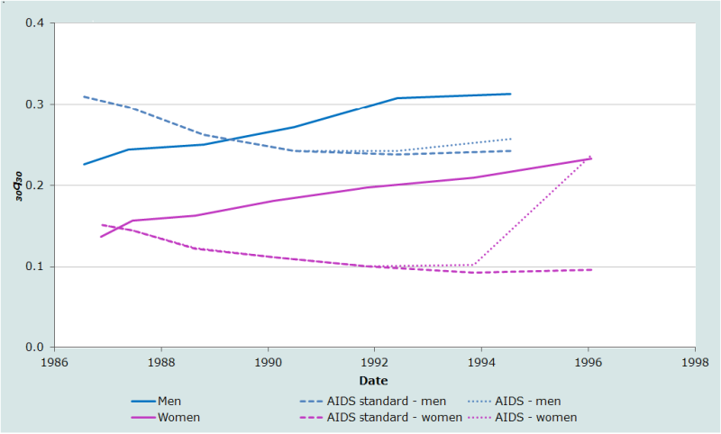
To use the UN General model to estimate ₃₀q₃₀ in Kenya for the 1990s amounts, in effect, to assuming that the rises in mortality from AIDS occurring among younger adults were matched by comparable rises in mortality among middle-aged individuals. This seems unlikely. The estimates of ₃₀q₃₀ made using the AIDS standards, in contrast, imply that any rise in the mortality of young adults was more than offset by continuing declines in the death rates of middle-aged adults in the late 1980s and more-or-less exactly offset by such declines till about 1993. However, few of the parents of respondents who were themselves in their thirties in 1999 are likely to have become infected with HIV and so using the AIDS standard to make the early estimates of ₃₀q₃₀ also seems inappropriate. Perhaps the most likely scenario is that the probability of dying between ages 30 and 60 stagnated between the late-1980s and mid-1990s and then began to rise, though probably somewhat less abruptly than is indicated by the ‘AIDS’ series for women.

The crucial point to emphasize is that it is impossible to determine from these data exactly what happened to adult mortality in Kenya in the 1990s. The only estimates that are fairly reliable are those for the late 1980s. These results are based on age groups for which only limited adjustment of the proportions of parents that are alive is needed to estimate ₃₀q₃₀. Thus, the series based on different standards intersect at this time.

Orphanhood before and since marriage

Methods exist for estimating adult mortality from orphanhood that can be used when supplementary questions are asked in a single survey about the timing of the deaths of parents relative to first marriage (Timæus 1991). Two aims underlie these methods. The first is to produce methods with a more specific and up-to-date time reference than those yielded by the original method. The second is to develop methods that are less subject to bias due to under-reporting of orphanhood at young ages.

Marriage is an event that distinguishes, for each age group of respon­dents, more recent parental deaths from those that occurred longer ago. While the inform­ation on the timing of deaths is less precise than that yielded by direct questions about the date of death of parents, it may be more accurately reported. Even if respondents cannot remember exactly when their parents died, it seems likely that nearly all of them will be able to report the timing of parental deaths relative to their first marriage, another event of major significance in their lives.

Some 15 inquiries conducted as part of Phase 1 of the Demographic and Health Surveys programme collected data on the relative timing of the deaths of parents and first marriage. Unfortunately, few or no surveys have done so more recently. Data on the timing of first births relative to the birth of respondents’ first child could be analysed in exactly the same way and might be more representative of the mortality of all parents in populations in which many people never marry or in which getting married is thought of as a process rather than an event that occurs on a well-defined date.

Because men and women marry (and have their first births) at different ages, the reports of male and female respondent should be analyzed separately. The estimation coefficients discussed here were developed primarily for the analysis of data supplied by female respondents (Timæus 1991) but could also be used for the analysis of data supplied by men if their mean age at marriage is less than 25. For respondents whose age exceeds the mean age at marriage, the estimates are robust to any characteristics of the distribution of ages of marriage other than its mean.

Orphanhood since first marriage

The proportion of mothers that have remained alive since respon­dents married is closely related to the probability of surviving from the sum of the period mean age at childbearing and the cohort mean age at marriage until the sum of the mean age at childbearing and the current age of the respondents. Estimates made from data on orphanhood since marriage will measure more recent mortality than those based on respondents' lifetime experience of orphanhood. In addition, because parental deaths since marriage must have occurred when respondents were sufficiently old to remember them clearly, such data could be less subject to reporting errors than those concerning the overall level of orphanhood.

The earliest central age of respondents (n) for which one can estimate a survivorship ratio, _np_b, from data on orphan­hood since marriage is 30 years. For women, to preserve a close relationship between maternal survival and life table survivorship, the latter is measured from a base age, b, of 45 years. Thus, the model used to estimate life table measures from the survival of mothers since the respondents married is:

$${}_{n-20}p{}_{45}=a(n)+b(n){\overline{M}}^f+c(n)\overline{m}+d(n){}_{5}S{}_{n-5}/{}_{5}S{}_{n-5}^m+e(n){}_{5}S{}_n/{}_{5}S{}_n^m$$

where $$\overline{m}$$ is the cohort mean age at marriage and $${}_{5}S{}_n^m$$ is the proportion of respondents in age group n to n+5 who at the time of their first marriage had living mothers.

The only difference in the equation for the estimation of men’s mortality from paternal orphanhood since marriage arises from the fact that men tend to be older than women at the birth of their children. Therefore, survivorship is estimated from a base age that is 10 years greater. The estimates are made using:

$${}_{n-20}p{}_{55}=a(n)+b(n){\overline{M}}^m+c(n)\overline{m}+d(n){}_{5}S{}_{n-5}/{}_{5}S{}_{n-5}^m+e(n){}_{5}S{}_n/{}_{5}S{}_n^m$$

where the age at marriage referred to is still that of the respondents, who will usually be female, not the parents, who are now male.

Until most respondents have married, the relationship between life table survivorship and the proportions of parents alive is sensitive to the shape of the age distribution of first marriages. Thus, coefficients exist for estimating survivorship over the age ranges ₁₀p₄₅ to ₃₀p₄₅ for adult women and ₁₀p₅₅ to ₂₀p₅₅ for adult men (see Table 8).

Table 8 Coefficients for estimating adult women’s and men’s mortality from orphanhood since first marriage

n	a(n)	b(n)	c(n)	d(n)	e(n)
Adult women
30	0.5617	0.00836	-0.00261	-1.1231	1.4199
35	0.0476	0.01396	-0.00536	-0.3916	1.1354
40	-0.3715	0.01966	-0.00744	0.5394	0.5286
45	-0.6562	0.02587	-0.00716	1.0208	0.1789
50	-0.8341	0.03045	-0.00561	1.1898	0.0541
Adult men
30	0.0676	0.01588	-0.00633	-1.2070	1.8284
35	-0.5459	0.02273	-0.01083	-0.2509	1.3867
40	-0.8674	0.02622	-0.01135	0.6057	0.7198
Source: Timæus (1991)

Orphanhood before first marriage

The proportion of women with living mothers at marriage approximately equals the life table probability of surviving from the mean age at childbearing of the mothers to that age plus the mean age at first marriage of their daughters. If the data are not biased by the adoption effect, this variant on the orphanhood method has two valuable characteristics. First, it measures mortality over a limited and fairly clearly defined interval of time and range of ages. Secondly, the estimates are capable of extending the time series of mortality estimates provided by the orphanhood method backward to at least 30 or 35 years before the data were collected.

For orphanhood before marriage an interaction term between the mean age at marriage and proportion orphaned improves the fit of the model. Thus, the probability of surviving from age 25 to age 45 for women can be estimated from orphanhood before marriage using the regression equation:

$${}_{20}p{}_{25}=a(n)+b(n){\overline{M}}^f+c(n)\overline{m}+d(n){}_{5}S{}_n^m+e(n)\overline{m}{}_{5}S{}_n^m$$

The coefficients of this equation for the different age groups defined by n are presented in Table 9.

The same considerations apply to the estimation of adult male mortality from paternal orphanhood before marriage. Estimates of the probability of surviving from age 35 to age 55 are made from:

$${}_{20}p{}_{35}=a(n)+b(n){\overline{M}}^f+c(n)\overline{m}+d(n){}_{5}S{}_n^m+e(n)\overline{m}{}_{5}S{}_n^m$$

These coefficients are also presented in Table 9.

Table 9 Coefficients for estimating adult women’s and men’s mortality from orphanhood before first marriage

n	a(n)	b(n)	c(n)	d(n)	e(n)
Adult women
30	-0.9607	0.00418	0.04466	-0.04291	1.8178
35	-0.9921	0.00429	0.04700	-0.04501	1.8428
40	-1.0129	0.00433	0.04822	-0.04611	1.8607
45	-1.0206	0.00434	0.04861	-0.04648	1.8680
Adult men
30	-1.2719	0.01060	0.04480	-0.04007	1.8383
35	-1.2977	0.01068	0.04652	-0.04124	1.8530
40	-1.3203	0.01070	0.04769	-0.04225	1.8726
45	-1.3232	0.01070	0.04783	-0.04238	1.8753
Source: Timæus (1991)

For orphanhood before marriage, the final sets of coefficients presented for maternal and paternal orphanhood before marriage in Table 9 refer to an age group in which first marriage is almost complete. These coefficients can be used to estimate mortality from the reports of any age group of respondents aged 40 and above. Only the accuracy of reporting about parental deaths and respondents' own ages impose an upper age limit on the data on orphanhood before marriage that can be used to estimate mortality.

Time location of the estimates

Like those from lifetime orphanhood, estimates made from the data supplied by different age cohorts of respondents, about orphanhood before and after marriage, reflect mortality over varying and ill-defined periods of time. For orphanhood before marriage, the time reference of the mortality measures is the product of the distribution of intervals between parental deaths and marriage and the distribution of intervals between marriage and interview. To the degree of precision required, the time reference of maternal orphanhood estimates is the average interval from orphanhood to first marriage plus the average interval from first marriage to interview. For cohorts of women who have nearly all married, the ages at which the parents are exposed to the risk of dying are concentrated between their mean age at childbearing and the sum of that age and their daughters' mean age at first marriage. The time reference of the mortality measures can be calculated as:

$$T=(N-\overline{m})+{}_{\overline{m}}g{}_{\overline{M}}$$

The second term on the right-hand side of equation 5 can be estimated using the procedure explained with reference to the basic method (see Step 4). As for lifetime orphanhood, the time reference of estimates of male mortality should allow for deaths between conception and birth and are calculated using $${}_{\overline{m}+0.75}g{}_{\overline{M}-0.75}$$.

For orphanhood since marriage, the age at which parents enter exposure to the risk of death is the product of their distribution of ages at childbearing and their daughters’ ages at marriage. For age groups that have largely completed marriage, one can estimate the mean age at which exposure starts as the sum of the means of these two distributions. The parents’ exposure continues till the time of interview, $$N-\overline{m}$$ years later. Thus, the time references of the mortality measures are:

$$T={}_{N-\overline{m}}g{}_{\overline{M}+\overline{m}}$$

Because the age range over which fathers are exposed to the risk of death commences well after the birth of their daughters, this equation is appropriate for estimates of both men’s and women’s mortality.

Illustrative application

Figure 3 portrays the results of the application of the orphanhood before and since first marriage method for estimating adult mortality to data collected from women aged 15 to 49 in the 1988 Demographic and Health Survey (DHS) of Egypt. The first striking feature of these results is that the information on whether the older respondents were orphans when they first married collected in 1988 generates a series of estimates of adult mortality that extends back to the early 1950s. Second, the additional sets of estimates produced by partitioning the orphaned women into those who were orphaned before they first married and those who have been orphaned since, tie in consistently with those produced from data on lifetime orphanhood. These results offer no evidence that the underreporting of orphanhood due to the adoption effect is biasing down the most recent estimates based on lifetime orphanhood or those based on orphanhood before first marriage.

 

Image

Figure 3 Trends in the probability of dying between exact ages 30 and 60 estimated from orphanhood, Egypt, 1988 Demographic and Health Survey

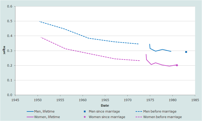
According to these results, a steady, gradually decelerating drop in adult mortality occurred in Egypt between the early-1950s and mid-1980s. The probability of dying between exact ages 30 and 60 fell by about 200 per thousand over this period for both men and women from a very high level in the early 1950s to about 200 per thousand for women and 300 per thousand for men in the early 1980s. Even these most recent estimates represent rather high mortality. The 100 per thousand difference between the probabilities of dying of men and women changed hardly at all over the period. The orphanhood estimates of adult mortality for men, in particular, are substantially higher than those based on other sources (UN Population Division 2011).

Questions about the timing of parental deaths

A further extension to the orphanhood method is to ask respondents whose parents have died about when the death occurred (Chackiel and Orellana 1985). If the dates on which parents died are reported with reasonable accuracy, this enables the analyst to distinguish recent from more distant parental deaths and obtain more up-to-date estimates of mortality. The best way to analyze such data is to use the information on dates of death to reconstruct the proportion of respondents who had living parents five and ten years earlier. From these successive cross-sections, one can construct synthetic cohort measures of parental survival that are formally identical to those generated from data collected in a series of separate inquiries. Therefore, methods for the analysis of these data are discussed jointly with the analysis of orphanhood data from multiple inquiries.

Further reading and references

The orphanhood method is discussed in all the classic manuals on indirect estimation (Sloggett, Brass, Eldridge et al. 1994; UN Population Division 1983) but, with the exception of the United Nations’ manual on estimating adult mortality (United Nations Population Division 2002), these manuals give emphasis to the older variant of the method that uses weighting factors to produce life table indices, rather than the regression-based method normally used today. Although regression-based methods for women had been proposed previously (Hill and Trussell 1977; Palloni and Heligman 1985), regression methods for estimating men’s mortality were first developed by Timæus (1992). His article also surveys earlier contributions to the literature and discusses the theoretical basis of the method.

Methods for estimating adult mortality from orphanhood before and after marriage are described in Timæus (1991). Procedures for estimating women’s mortality in populations experiencing generalized HIV epidemics were developed by Timæus and Nunn (1997).

Luy (2012) has proposed a modified orphanhood method intended for the study of socio-economic differentials in adult mortality in countries that already have accurate aggregate information on adult mortality. His method determines the relationship between the proportion of survey respondents reporting living parents and life table survivorship from empirical statistics on the population concerned instead of using demographic models. Thus, Luy’s method tailors the estimation process to the context. Few low- and middle-income countries have sufficiently accurate national data for this to be feasible, though aspects of the approach may be of relevance in some circumstances.

Methods that exploit the additional analytic opportunities that arise when questions about orphanhood have been asked in two or more successive inquiries in the same population are discussed elsewhere in this manual.

 

Blacker JGC. 1984. "Experiences in the use of special mortality questions in multi-purpose surveys: the single-round approach," in Data Bases for Mortality Measurement. New York: United Nations, pp. 79-89. https://www.un.org/development/desa/pd/sites/www.un.org.development.desa.pd/files/publications/mortality/mortality_1984_databasesformortalitymeasurements.pdf

Blacker JGC and JM Gapere. 1988. “The indirect measurement of adult mortality in Africa: results and prospects,” in African Population Conference, Dakar, 1988. Liège: International Union for the Scientific Study of Population,Vol. 2:3.2.23–38.

Brass W. 1971. "On the scale of mortality," in Brass, W (ed). Biological Aspects of Demography. London: Taylor and Francis, pp. 69-110.

Brass W. 1975. Methods for Estimating Fertility and Mortality from Limited and Defective Data. Chapel Hill: International Program of Laboratories for Population Statistics.

Brass W. 1985. Advances in Methods for Estimating Fertility and Mortality from Limited and Defective Data. London: London School of Hygiene & Tropical Medicine.

Brass W and EA Bamgboye. 1981. The Time Location of Reports of Survivorship: Estimates for Maternal and Paternal Orphanhood and the Ever-widowed. London: London School of Hygiene & Tropical Medicine.

Brass W and K  Hill. 1973. “Estimating adult mortality from orphanhood,” in International Population Conference, Liège, 1973. Liège: International Union for the Scientific Study of Population, Vol. 3:111–123.

Chackiel J and H Orellana. 1985. “Adult female mortality trends from retrospective questions about maternal orphanhood included in censuses and surveys,” in International Population Conference, Florence, 1985. Liège: International Union for the Scientific Study of Population, Vol. 4:39–51.

Chen W-J and N Walker. 2010. "Fertility of HIV-infected women: insights from Demographic and Health Surveys", Sexually Transmitted Infections 86(Suppl 2):ii22-ii27. doi: https://dx.doi.org/10.1136/sti.2010.043620

De Cock KM, MG Fowler, E Mercier, I de Vincenzi et al. 2000. "Prevention of Mother-to-Child HIV Transmission in Resource-Poor Countries", Journal of the American Medical Association 283(9):1175-1182. doi: https://dx.doi.org/10.1001/jama.283.9.1175

de Walque D. 2007. "Sero-discordant couples in five African countries: implications for prevention strategies", Population and Development Review 33(3):501-523. doi: https://dx.doi.org/10.1111/j.1728-4457.2007.00182.x

Freeman EE and JR Glynn. 2004. "Factors affecting HIV concordancy in married couples in four African cities", AIDS 18(12):1715-1721. doi: https://dx.doi.org/10.1097/01.aids.0000139075.13906.2f

Henry L. 1960. "Mesure indirecte de la mortalité des adultes", Population 15:457-466.

Hill K. 1984. "An evaluation of indirect methods for estimating mortality," in Vallin, J, Pollard John H and L Heligman (eds). Methodologies for the Collection and Analysis of Mortality Data. Liège: Ordina, pp. 145-176.

Hill K and TJ Trussell. 1977. "Further developments in indirect mortality estimation", Population Studies 31(2):313-334. doi: https://dx.doi.org/10.2307/2173920

Kaiser R, R Bunnell, A Hightower, AA Kim et al. 2011. "Factors Associated with HIV Infection in Married or Cohabitating Couples in Kenya: Results from a Nationally Representative Study", PLoS ONE 6(3):e17842. doi: https://dx.doi.org/10.1371%2Fjournal.pone.0017842

Luy M. 2012. "Estimating mortality differences in developed countries from survey information on maternal and paternal orphanhood", Demography 49(2):607-627. doi: https://dx.doi.org/10.1007/s13524-012-0101-4

Mahy M, J Stover, K Kiragu, C Hayashi et al. 2010. "What will it take to achieve virtual elimination of mother-to-child transmission of HIV? An assessment of current progress and future needs", Sexually Transmitted Infections 86(Suppl 2):ii48-ii55. doi: https://dx.doi.org/10.1136/sti.2010.045989

Palloni A and L Heligman. 1985. "Re-estimation of structural parameters to obtain estimates of mortality in developing countries", Population Bulletin of The United Nations 18:10-33. https://www.un.org/development/desa/pd/sites/www.un.org.development.desa.pd/files/files/documents/2020/Jan/un_1986_population_bulletin_18.pdf

Palloni A, M Massagli and J Marcotte. 1984. "Estimating adult mortality with maternal orphanhood data: analysis of sensitivity of the techniques", Population Studies 38(2):255-279. doi: https://dx.doi.org/10.1080/00324728.1984.10410289

Sloggett A, W Brass, SM Eldridge, IM Timæus, P Ward and B Zaba. 1994. Estimation of Demographic Parameters from Census Data. Tokyo, Japan: United Nations Statistical Institute for Asia and the Pacific.

Timæus I. 1986. "An assessment of methods for estimating adult mortality from two sets of data on maternal orphanhood", Demography 23(3):435-450. doi: https://dx.doi.org/10.2307/2061440

Timæus IM. 1991. "Estimation of adult mortality from orphanhood before and since marriage", Population Studies 45(3):455-472. doi: https://dx.doi.org/10.1080/0032472031000145636

Timæus IM. 1992. "Estimation of adult mortality from paternal orphanhood: a reassessment and a new approach", Population Bulletin of The United Nations 33:47-63. https://www.un.org/development/desa/pd/sites/www.un.org.development.desa.pd/files/files/documents/2020/Jan/un_1992_population_bulletin_33.pdf

Timæus IM and AJ Nunn. 1997. "Measurement of adult mortality in populations affected by AIDS: an assessment of the orphanhood method", Health Transition Review 7(Suppl 2):23-43. https://www.jstor.org/stable/40652324

UN Population Division. 1983. Manual X: Indirect Techniques for Demographic Estimation. New York: United Nations, Department of Economic and Social Affairs, ST/ESA/SER.A/81. https://www.un.org/esa/population/techcoop/DemEst/manual10/manual10.html

UN Population Division. 2002. Methods for Estimating Adult Mortality. New York: United Nations, Department of Economic and Social Affairs, ESA/P/WP.175. https://www.un.org/development/desa/pd/sites/www.un.org.development.desa.pd/files/files/documents/2020/Jan/un_2002_methodsestimatingadultmort.pdf

UN Population Division. 2011. World Mortality Report 2007. New York: United Nations, Department of Economic and Social Affairs, ST/ESA/SER.A/289. https://www.un.org/development/desa/pd/sites/www.un.org.development.desa.pd/files/files/documents/2020/Jan/un_2007_worldmortalityreport.pdf