Fertility estimation from cohort parity increments
Description of the method
Data on children ever born tabulated by standard 5-year age group of women for a single census or survey convey a lot of information about the past fertility experience of the women. Unfortunately, however, if fertility has been changing, it is not possible to use the average parities of women in different age groups to obtain estimates of the age patterns of either cohort or period fertility.
If information on children ever born is available from two censuses or surveys approximately five or 10 years apart, the change in the average number of children ever born by a particular cohort of women reflects their intercensal fertility. It then becomes possible to estimate an age-specific fertility schedule for the intervening period. Arretx (1973) developed a method for using such information with a 10-year interval between the inquiries. Manual X (UN Population Division 1983) presents a variant of an approach proposed by Coale and Trussell using the P/F ratio. A further refinement of the Manual X approach is presented here, based on the use of the relational Gompertz model.
The method estimates the average age-specific fertility rates in effect during the inter-survey period by constructing the average parities of a hypothetical, inter-survey cohort. A cumulated fertility schedule is then derived from these parities by interpolation, and age-specific fertility rates are obtained from cumulated fertility by successive subtraction.
The method is intended for situations in which it is possible to calculate average parities by age group of women for two points in time approximately five or 10 years apart. If the interval between the inquiries is five years, the women in any five-year age group at the second inquiry represent the survivors of the women in the next younger five-year age group at the first inquiry. The difference in the average parity of the cohort between the first and the second inquiries reflects its childbearing experience between the two inquiries, if it is assumed that women who died or migrated between them had, on average, lifetime fertility that was not systematically different from that of the original women who remained. By cumulating the parity increments, it is possible to estimate average parities for a synthetic cohort experiencing throughout its hypothetical lifetime the age-specific fertility rates in effect during the period between the two inquiries. If the length of this period is 10 years, a five-year age group at the second inquiry represents the survivors of the five-year age group who were two groups younger at the first inquiry. In this case, it is still possible to calculate the cohort parity increment for each cohort in order to construct the average parities of a hypothetical cohort. The method may be applied when the data come entirely or partially from nationally representative sample surveys as well as when they come from censuses, for although cohorts of particular individuals will not be identical on each occasion, their average parities will be representative of those of the sampled female population.
The two data sets need not refer to two points exactly five or 10 years apart. For example, unless fertility is changing very rapidly, a four-year interval or an 11-year interval will provide reasonable estimates. In such a case, one is no longer following a cohort from survey to survey, but this factor is not very important because the average parity of an age group will not change rapidly from one year to the next.
Although the strength of method lies in its robustness to changing fertility, the technique presented here can also be used to estimate age-specific fertility rates using parity data from a single census or survey when fertility has not been changing during the reproductive life spans of the women concerned.
Assumptions
Most of the assumptions are those associated with the relational Gompertz model, namely
- The standard fertility schedule chosen for use in the fitting procedure appropriately reflects the shape of the fertility distribution in the population.
- Any changes in fertility have been smooth and gradual and have affected all age groups in a broadly similar way.
- The parities reported by younger women in their twenties are accurate.
Further, in deriving this measure of inter-survey fertility it is assumed that mortality and migration have no effect on actual parity distributions; that is, it is assumed that the average parity of those women who die or migrate between the surveys is not significantly different from the average parity at comparable ages of those women who are alive and present at the end of the period.
Preparatory work and preliminary investigations
Before commencing analysis of fertility levels using this method, analysts should investigate the quality of the data at least in respect of the following dimensions:
- age and sex structure of the population; and
- average parities and whether an el-Badry correction is necessary.
Caveats and warnings
The general warning given about the use of information on children ever born in estimating fertility should be kept in mind in this instance. A tendency exists, even in countries with otherwise reasonably good data, for older women to omit some of their children, perhaps those who have died or those who have left home. As a result, average parities often fail to increase at a plausible rate, or may even decrease after age 35 or 40. The calculation of age-specific fertility rates from parities that suffer from such omissions will result in under-estimates of the fertility of older women. If the error is relatively minor, its effects may not be obvious. Thus, fertility estimates based on average parities of older women must be interpreted with caution, particularly if they indicate low fertility in relation to that estimated from the reports of younger women. Average parities for a hypothetical cohort are, moreover, very sensitive to changes in parity reporting from one inquiry to the other, and the calculation of such parities provides a useful consistency check of the raw data.
Whenever the additional data required on recent fertility exist, the procedure using a synthetic relational Gompertz model to compare cumulated intersurvey fertility rates with hypothetical-cohort average parities is to be preferred to the method described here, since the former method is less sensitive to the omission of children ever born from the reports of older women.
Application of the method
Steps 1 and 2 simply repeat the first two steps of the synthetic relational Gompertz method.
Step 1: Calculation of reported average parities from each inquiry
Calculate the average parities, and of women in each age group [x,x + 5) for the two inquiries (t1 and t2), for x =15, 20 … 45 if not already done as part of the preliminary investigations, or produced as a consequence of applying the el-Badry correction. For ease of exposition, we denote the average parity in age group i at time t by where i= (x/5 - 2). Thus, the average parities obtained from the first census or survey are denoted by P(i,1), and those from the second inquiry by P(i,2).
Step 2: Calculation of average parities for a hypothetical cohort
The way in which the parities are calculated depends upon the length of the interval between the two inquiries.
a) Interval is of five years’ duration
If the interval between the two data series is five years, all the survivors of age group i at the first inquiry are in age group i+1 at the second inquiry, and the parity increment between the inquiries for the corresponding cohort is equal to P(i+1,2) - P(i,1). Such increments can be calculated for each age group, and the hypothetical-cohort parities are then obtained by successively cumulating them. Thus, if the parity increment for the cohort of age group i at the first inquiry is denoted by , and the parity of age group i for the hypothetical cohort is denoted by P(i,s) (where the s stands for 'synthetic'), one has for i=1…6, and hence
.
The parity increment for the youngest age group (i = 0) is taken as being equal to P(1,2), i.e., assuming that P(0,1), the average parities of women aged 10-14 in the first inquiry, is zero. If fertility is changing rapidly, this value of will therefore reflect period rates somewhat closer to the inquiry survey than to the mid-point of the interval, slightly over-allowing for the change in fertility.
b) Interval is of ten years’ duration
If the intercensal or inter-survey period is 10 years, then the survivors of the initial cohort of age group i in the first survey will be the women in age group (i+2) in the second. Hypothetical cohort parities are then obtained by cumulating two parallel sequences of parity increments. Once more, for the youngest age groups, is taken as being equal to P(1,2) and to P(2,2). Other parity increments are calculated as for i=1…5.
Hypothetical-cohort parities for even-numbered age groups are obtained by summing the parity increments for even-numbered age groups, whereas those for odd- numbered age groups are obtained by summing parity increments for odd-numbered age groups. Thus,
.
The following steps repeat those involved in using the relational Gompertz model, but fit a line only to the parity data.
Step 3: Fitting of a relational Gompertz model
If the parity data are internally consistent, the plots of z(i) - e(i) against g(i) should result in straight lines. Those P-points that cause the plot to deviate from a straight line should be excluded from the model. Ordinary linear regression (using least squares) is used to fit lines to the P-points and to identify, sequentially, those points that do not fit neatly on a straight line. The intention is to seek the most numerous combination of P-points that lie (almost) on the same line, and to use these to fit the model.
Points are selected for inclusion using the following guidelines:
- A contiguous series of points must be included in the model. Sequentially, only the end-most points can be excluded. (The reason for this is that each point on the graph is the result of calculations involving the ratio of a pair of adjacent data values. If the analysis leads to the conclusion that a data value is unreliable as a denominator of one of these ratios it is not logical to then accept it as the numerator of the next ratio.)
- P-points at older ages should be eliminated in preference to those at younger ages since data at these ages are usually the least reliable and exhibit the least consistency between lifetime and recent fertility.
- Where only a marginally worse fit is achieved with more points, this is to be preferred to a slightly better fit achieved with fewer points.
Step 4: Assess the fitted parameters
The values of α and β that represent the best-fitting line joining the remaining P-points and F-points must be checked to ascertain that they are not so far from their central values as to suggest that the standard chosen is inappropriate. A good fit is indicated if -0.3 < α < 0.3, and if 0.8 < β < 1.25.
If the parameters lie outside this range, one or both of the underlying data series are problematic or the standard is inappropriate. Experimentation with another standard or changing the selection of points should be done before proceeding further. If the parameters still lie outside the ranges above, the method should be regarded as inappropriate.
Step 5: Fitted ASFRs and total fertility
Having estimated the two parameters of the model, they can be applied to the standard values for the parities to obtain fitted values, .
These are then converted back into measures of the cumulative proportion of fertility achieved by age group i using the anti-gompit transformation. The anti-gompits based on the parity distributions indicate the proportion of fertility achieved by that age group. Dividing observed parity in each age group by these proportions produces a series of estimates of total fertility. Averaging these values across the sub-set of age groups that were used to estimate α and β gives the fitted estimate of total fertility, .
Applying the same α and β to the standard gompits for the ages that divide conventional age groups (i.e. 20, 25 … 50), applying the anti-gompit transformation, and multiplying by produces a scaled cumulated fertility schedule. Differencing successive estimates of cumulated fertility and dividing by five produces the fitted fertility schedule for conventional age groups (15-19; 20-24 etc.).
These ASFRs are then deemed to apply to the mid-point of the period in between the two inquiries.
Worked example
The example uses the same data on average parities from the 1989 and 1999 censues of Kenya as in the example of the synthetic relational Gompertz model. In this application, however, it is assumed that the only available information is the average parities and that no data on recent fertility were collected. The process of fitting the relational Gompertz model to parity data alone is essentially similar to the basic relational Gompertz model. The exposition here therefore concentrates on the differences from that procedure. The method has been implemented in an accompanying Excel workbook.
Step 1: Calculation of reported average parities from each inquiry
An el-Badry correction was applied to the data from the 1989 census. Its application is described here. By contrast, the data from the 1999 census had evidently been edited, and no missing parity data were present. The average parities from the two censuses are shown in the first two columns of Table 1. From these data, it would appear that the cohort lifetime fertility of older women has fallen by around 0.6 of a child over that decade. However, the increase in lifetime fertility among teenaged women is somewhat surprising.
Step 2: Calculation of average parities for a hypothetical cohort
The inter-survey period is 10 years (from 1989 to 1999). We therefore use the routine described in Step 2(b) to derive the cohort average parities, shown in the last column of Table 1.
Table 1 Average parities by age group, Kenya, 1989 and 1999 Censuses
| Age group |
1989 |
1999 |
Hypothetical cohort parity P(i,s) |
|
15-19 |
0.2416 |
0.2848 |
0.2848 |
|
20-24 |
1.5247 |
1.3640 |
1.3640 |
|
25-29 |
3.2138 |
2.6073 |
2.6505 |
|
30-34 |
4.7602 |
4.1432 |
3.9825 |
|
35-39 |
6.2390 |
5.3867 |
4.8234 |
|
40-44 |
7.1204 |
6.3818 |
5.6041 |
|
45-49 |
7.5103 |
6.9143 |
5.4987 |
As described in Step 2(b), and , while
It is readily apparent that severe omissions of parities must have been present at older ages, as the hypothetical cohort parity at the oldest age group is somewhat lower than that of women in the hypothetical inter-survey cohort aged 40-44.
The definition of the age of the mother does not enter into this method. Average parities are – by definition – those prevailing at the survey or census date.
Step 3: Fitting of a relational Gompertz model
The hypothetical cohort data in the last column of Table 1 are used to estimate fertility by means of the relational Gompertz model. Data points based on the average parities (P-points) are successively eliminated until the data points show a linear relationship with the (transformed) parities from the standard fertility schedule. The fitted points are shown in Figure 1.
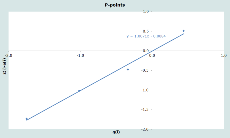
Only five parity points can be plotted as the hypothetical parity for the 45-49 age group is lower than that of the 40-44 age group (5.4987 vs. 5.6041), meaning that the gompit of the ratio of this pair of points is undefined. Examining the points, there is evident under-reporting of fertility in the ages used to generate the last point plotted. Eliminating that point results in a much lower root mean square error, and the model is fitted to the remaining four points.
Step 4: Assess the fitted parameters
The implied values of α and β are -0.0084 and 1.0071 implying a fertility schedule fairly close to that underlying the modified Zaba standard.
Step 5: Fitted ASFRs and total fertility
Applying these parameters to the gompits of the parities in the standard using the linear relational model, , taking the anti-gompits (column 4 of Table 2) and dividing these into the observed parities at the ages selected for inclusion in the model produces a series of five estimates of total fertility (ranging from 5.4 to 5.7 children per woman). Averaging these suggests total fertility () is 5.54 children per woman.
Table 2 Derivation of estimated total fertility (T-hat), Kenya, 1989 and 1999 Censuses
|
Age (i) |
Ys(i) |
Fitted Y(i) |
exp(-exp(-Y(i))) |
Actual cumulant |
|
0 |
-2.0961 |
-2.1194 |
0.0002 |
0.0013 |
|
1 |
-1.0833 |
-1.0994 |
0.0497 |
0.2754 |
|
2 |
-0.3124 |
-0.3230 |
0.2513 |
1.3930 |
|
3 |
0.3541 |
0.3482 |
0.4936 |
2.7368 |
|
4 |
1.0579 |
1.0570 |
0.7065 |
3.9166 |
|
5 |
1.9561 |
1.9615 |
0.8688 |
4.8167 |
|
6 |
3.4225 |
3.4384 |
0.9684 |
5.3688 |
|
7 |
6.0922 |
6.1270 |
0.9978 |
5.5320 |
Applying the fitted estimates of α and β to the standard gompits, Ys(x), in each age group to derive the fitted gompits,, then taking the anti-gompits and multiplying up by produces the modified cumulative fertility schedule, FM(x), below. Differencing and dividing by five produces the final schedule of age-specific fertility rates in the last column of Table 3.
Table 3 Derivation of final adjusted fertility schedule, Kenya, 1989 and 1999 Censuses
|
Age (x) |
Ys(x) |
Fitted Y(x) |
exp(-exp(-Y(i))) |
FM(x) |
fm(x) |
|
15 |
-1.7731 |
-1.7262 |
0.0036 |
0.0212 |
0.0042 |
|
20 |
-0.6913 |
-0.7318 |
0.1251 |
0.7318 |
0.1421 |
|
25 |
0.0256 |
-0.0727 |
0.3411 |
1.9957 |
0.2528 |
|
30 |
0.7000 |
0.5472 |
0.5607 |
3.2801 |
0.2569 |
|
35 |
1.4787 |
1.2630 |
0.7537 |
4.4090 |
0.2258 |
|
40 |
2.6260 |
2.3176 |
0.9062 |
5.3013 |
0.1785 |
|
45 |
4.8097 |
4.3249 |
0.9869 |
5.7732 |
0.0944 |
|
50 |
13.8155 |
12.6034 |
1.0000 |
5.8501 |
0.0154 |
|
Total Fertility |
|
|
|
|
5.53 |
The resulting estimate of total fertility is 5.53 children per woman, applicable half-way between the two censuses. In this application, the estimated age-specific fertility rates derived from the hypothetical-cohort parities can be compared with those obtained from the application of the synthetic relational Gompertz model (TFR = 5.56 children per woman). The similarity of the two sets of results is reassuring.
It must be remembered, however, that the results can be seriously distorted if children ever born tend to be omitted from the reports provided by their mothers, particularly if the extent of such omission changes from one survey to the next.
Detailed description of method
The method described here is simply a variant of the relational Gompertz model, but instead of using parity and fertility data collected at one point in time, constructs an 'average' fertility schedule based on reports of lifetime fertility at two points in time and uses these – alone – to determine a fertility schedule. The mathematics of the relational Gompertz model is described fully here.
Variants of the method
An option in the spreadsheet allows the intercensal period to be set to zero. This allows the derivation of a total fertility from one set of parity data alone. For this procedure to yield plausible estimates, not only would the average parities would have to be without error, but fertility would have had to have been constant for an extended period of time preceding the inquiry.
Further reading and references
The basic mechanics of the method were set out by Arretx (1973) and written up in Manual X (UN Population Division 1983). The version in Manual X used the P/F ratio method to convert the parity increments into fertility rates; the method here uses the more versatile relational Gompertz method.
Arretx C. 1973. "Fertility estimates derived from information on children ever born using data from censuses," in International Population Conference, Liège 1973. Vol. 2. Liège: International Union for the Scientific Study of Population, pp. 247-261.
UN Population Division. 1983. Manual X: Indirect Techniques for Demographic Estimation. New York: United Nations, Department of Economic and Social Affairs, ST/ESA/SER.A/81. https://www.un.org/development/desa/pd/sites/www.un.org.development.desa.pd/files/files/documents/2020/Jan/un_1983_manual_x_-_indirect_techniques_for_demographic_estimation.pdf
- Printer-friendly version
- Log in to post comments