Direct estimation of fertility from survey data containing birth histories
Description of method
The direct estimation of fertility (age-specific, and total) from survey data containing birth histories is relatively straightforward. If the data are carefully collected with a validated instrument (such as that used by the Demographic and Health Surveys), they can provide reliable and accurate estimates of fertility. However, distortions also frequently occur in birth history data, especially in relation to the shifting of births to more distant years to avoid additional questions on, for example, child health or anthropometry (Cleland 1996). These problems have again been highlighted recently by Schoumaker (2010, 2011). Displacement and omission of births might cause fertility (particularly in the period three to five years before the survey) to be underestimated.
Two approaches can be used to estimate fertility directly from data containing a detailed birth history. The first approach – that used by the DHS in its official reports – produces an estimate covering the one- or three-year period before the survey. (Three-year estimates are frequently used to avoid undesirable fluctuations in the estimates arising from the relatively small number of annual births in the DHS). This approach, is described in detail in the Guide to DHS Statistics (Rutstein and Rojas 2003). There are two disadvantages to it. First, if the survey is carried out over an extended period, it becomes impossible to locate the measure of fertility precisely in time. Second, the calculation of fertility rates is made more complex both by having to refer to the survey date and by working in five-year age groups and three-year periods of calendar time.
The simpler approach described here produces estimates of fertility for individual ages and calendar years of time. These can be very easily aggregated to produce estimates for wider age groups, or for periods of several years.
As with the DHS approach, initial manipulations have to be performed at a unit record level. For this reason, it makes sense in almost all circumstances, to estimate fertility directly from birth histories using the built-in survival time functionality of a statistical analysis program such as Stata. A useful routine for performing these calculations in Stata has been produced by Schoumaker (2013). However, the calculations are sufficiently straightforward to carry out using simple cross-tabulations of data. This section describes how.
Data requirements and assumptions
Data required
Two sets of data, both routinely produced at the data processing stage of a survey with detailed birth histories, are required. The first is a data set in which the unit of analysis is the woman – i.e. there is one record per woman. These data are required to estimate the denominator of the fertility rates. The second data set has the child as the unit of analysis – i.e. there is one record per child – but also includes essential information on the mother (crucially, her date of birth) in each record in the data set.
To estimate fertility, the following information must be present in the data.
a) Women’s data set
- The month and year of each woman’s birth, derived if necessary from a century-month code (CMC).
- The month and year of interview.
- Any variables needed to adjust the data for the sampling design and sample weights.
- Important covariates by which one might wish to assess differentials in fertility, bearing in mind that covariates at the date of interview may not have applied at the time the events of interest (recent births) took place.
b) Child’s data set
- The child’s date of birth – month and year, derived if necessary from a CMC.
- The mother’s date of birth – month and year, derived if necessary from a CMC.
- Any variables needed to adjust the data for the sampling design and sample weights.
- The same covariates by which differentials in fertility are to be assessed.
Caveats and warnings
- While single-age fertility rates derived from relatively small-scale surveys provide some indication of the quality of the data, the rates are almost always too erratic to be of direct use. Aggregation into five-year groups (and then – perhaps – smoothing the rates by means of a relational Gompertz model) is almost always called for.
- Similarly, rates for a single calendar year derived from survey data may not be reliable. Data for multiple calendar years should be combined to produce a more reliable estimate. However, ideally, one should not combine more than three years’ data to avoid flattening out the trend in fertility.
- The rates produced using this approach may be affected materially by omission or displacement of the date of reported births.
- The rates produced in this manner will not be the same as those produced by MeasureDHS. In the first place, the estimation of the period exposed to risk is a little different (MeasureDHS works in complete months, while here we work in half-months). Second, the reference period for the rates may differ by up to 11 months. One could, however, calculate rates for years running from July to June (and thus centred on 1 January, or indeed for any other 12-month period) by manipulating the numerator and denominator appropriately.
Application of method
We define the following terms:
- the child’s month of birth
- the child’s year of birth
- the mother’s month of birth
- the mother’s year of birth
- the month in which the mother is interviewed
- the year in which the mother is interviewed
- the total number of births to mothers aged x at the birth of their child in calendar year t
- the person-years of exposure to risk of women aged x in calendar year t.
The rates are calculated by means of the following steps. To avoid having to make additional assumptions about the exposure to risk in the month of interview, both exposure and births occurring in the month of interview are ignored.
The general case is presented below where not all women are interviewed in the same calendar year. Where all women are interviewed in the same calendar year, the process can be simplified accordingly.
Step 1: Produce a tabulation of the number of births in each calendar year by the age of the mother at the birth of the child
This step produces the numerator of the fertility rates: births of children by calendar year and age of mother at birth.
In principle, the tabulation is relatively straightforward, although care needs to be taken to allocate appropriately mother’s age at the birth of her child when both mother and child have the same month of birth. If, as is usually the case, information on day of birth is not available, it is necessary to allocate the mother’s day of birth randomly to fall before or after the child’s day of birth. This could be implemented by generating a binary variable, b, using a random number generator, but doing so would have implications for the consistency and replicability of investigations. Instead, b can be generated from a putatively uniform variable that has no bearing on the outcomes being investigated, such as the day of the month in which the mother was interviewed. We therefore define b= 1 if the day of interview is greater than 15, and 0 if the day of the month is 15 or less.
The age (at last birthday) of the mother at the birth of a given child, x, is given by
where int() represents the integer portion of the term in brackets.
Extract a tabulation showing the total number of births in each cell defined by combinations of and x, weighting the data as appropriate, and making sure to exclude births that occurred in the month that the mother was interviewed.
Step 2: Calculate the age of each woman at the start of the year in which she was interviewed
Working with the women’s data set (i.e. with one record per woman), begin by deriving the age of women on 1 January of the year of interview, xI, assuming that mothers’ births are uniformly distributed over calendar months (and hence occur, on average, half way through each month):
It follows that the age of the mother on 1 January of any other year, t, (t ≤ YI) will be xI - (YI - t).
Step 3: Calculate the exposed to risk for each woman in the year of her interview
In the calendar year in which she is interviewed, a woman is exposed to the risk of giving birth for only a portion of the year (that is, the portion before the interview takes place). In this case, the computation of exposure to risk depends critically on whether the interview took place before or after the woman’s birthday in that year. If her birth month precedes the interview month, she will be exposed to risk of giving birth at age xI for
years, and for
years at age xI+1. In contrast, if her birth month is the same as, or after, the month of her interview, her exposure to risk of giving birth in the year of interview will be for
years at age xI, and
years at age xI + 1.
Note that in the last complete year, aggregate exposure per woman is 1 year, whereas in the year of interview, aggregate exposure is (MI - 1)/12 of a year, regardless of the relative timing of birth month and interview month.
Variables giving each woman’s exposure at ages xI and xI + 1 in the year of interview must be derived, and then aggregated (weighting were necessary) to produce a tabulation of aggregate exposure by age in the year of interview.
Step 4a: Calculate the exposure to risk for each woman in the last complete calendar year before her interview
In the last complete calendar year before each woman is interviewed, i.e. in year t=YI - 1, she will be aged xI-1 until her birthday, and xI for the remainder of the year. On the same assumption as above of a uniform distribution of births within calendar months, the fraction of a year from 1 January until each woman’s birthday is given by
while for the remaining fraction of the year, she will be aged xI with exposure
.
Using the two formulae above, variables giving each woman’s exposure at ages xI and xI + 1 in year YI - 1 must be derived, and then aggregated (weighting were necessary) to produce a tabulation of aggregate exposure by age in that year.
Step 4b: Derive the exposure for earlier complete calendar years
Birth histories are collected retrospectively from all women and each woman provides information for the entire period over which she has been exposed to the risk of childbearing. Some women may have moved between places or changed their other characteristics at some point during this period but, because complete residential and economic histories are seldom collected in fertility surveys, it is usually impossible to allow for this when calculating fertility rates. This means that the interpretation of some results such as fertility by place of residence becomes less clear.
However, since birthdays are immutable, and the population of women being assessed is constant over time, the aggregate exposure of women attaining age x in a year for which all women’s exposure is complete, v, will also equal the exposure of the cohort in earlier years, that is:
Step 5: Derive the age-specific fertility rates
The total exposure at each age in each calendar year, E(x,t), is derived by summing the tabulations derived in steps 3 and 4 for each age and for each calendar year (complete and incomplete). Note that if fieldwork extends over two calendar years, YI -1 will refer to two different years, as will YI. Total exposure in the final calendar year for which exposure might be derived will be based on only the partial exposure of women interviewed in the final calendar year of fieldwork, whereas total exposure in the immediately preceding year will be comprised of the partial exposure of women interviewed in the first year of fieldwork and the full exposure in that year of women interviewed in the final year of fieldwork.
The age-specific fertility rates for age x in year t are given by
Age-specific fertility rates for conventional five-year age groups are derived by summing the births to women across each age group, and dividing by the sum of the exposure in that age group. Thus, if i=(x/5)-2 for x = 15, 20, …, 45, then
and
To combine data for multiple years, the numerators and denominators are summed separately before dividing to produce the rate:
Worked example
This example uses data from the 2004 Malawi DHS. Fieldwork in this survey began in earnest in October 2004 and ran through to February 2005.
Step 1: Produce a tabulation of the number of births in each calendar year by the age of the mother at the birth of the child
After random allocation of mother’s age at birth in cases where the mother and child’s month of birth are the same, the full cross tabulation of children’s year of birth by age of mother at the birth of her child is shown in Table 1. It would appear that there has been extreme shifting or omission of births in 2001 and 2002 in that the number of births reported in those years is some 20 per cent lower than that reported in 2003. Reported births in 2004 are lower than in 2003 in part because many women were not exposed for the full calendar year, and because births occurring in the month of interview are excluded from the analysis.
Table 1 Classification of births since 2001 by age of mother at birth, Malawi, 2004 DHS
|
|
Year of birth |
||||
|
Age |
2001 |
2002 |
2003 |
2004 |
2005 |
|
13 |
1.11 |
0.96 |
0.00 |
0.00 |
0.00 |
|
14 |
6.44 |
3.26 |
2.00 |
4.02 |
0.00 |
|
15 |
19.70 |
12.74 |
17.21 |
14.65 |
0.00 |
|
16 |
49.84 |
41.40 |
49.87 |
39.00 |
0.00 |
|
17 |
93.45 |
88.79 |
93.36 |
61.67 |
0.00 |
|
18 |
113.79 |
133.70 |
153.38 |
110.40 |
0.00 |
|
19 |
145.63 |
148.18 |
162.51 |
162.48 |
0.00 |
|
20 |
146.03 |
166.63 |
177.72 |
155.24 |
0.00 |
|
21 |
159.60 |
137.76 |
179.68 |
174.46 |
0.00 |
|
22 |
137.50 |
128.60 |
147.12 |
148.44 |
0.00 |
|
23 |
115.15 |
110.30 |
173.94 |
138.36 |
2.12 |
|
24 |
109.24 |
96.07 |
144.74 |
149.19 |
0.00 |
|
25 |
113.58 |
93.61 |
105.37 |
117.68 |
0.00 |
|
26 |
82.08 |
69.68 |
107.11 |
105.36 |
0.00 |
|
27 |
74.37 |
77.16 |
129.50 |
105.48 |
0.00 |
|
28 |
66.31 |
66.14 |
73.87 |
91.96 |
0.00 |
|
29 |
62.92 |
63.28 |
75.42 |
80.13 |
0.00 |
|
30 |
55.93 |
55.44 |
76.98 |
68.16 |
0.00 |
|
31 |
55.89 |
42.38 |
59.05 |
56.76 |
0.00 |
|
32 |
55.11 |
72.47 |
59.85 |
61.36 |
0.00 |
|
33 |
34.74 |
54.08 |
72.14 |
41.23 |
0.00 |
|
34 |
28.09 |
44.41 |
67.04 |
52.00 |
0.00 |
|
35 |
50.00 |
25.28 |
41.26 |
48.16 |
0.00 |
|
36 |
41.61 |
33.88 |
27.42 |
33.56 |
0.00 |
|
37 |
30.57 |
25.46 |
48.50 |
30.46 |
0.00 |
|
38 |
24.47 |
32.07 |
31.55 |
36.85 |
0.00 |
|
39 |
23.05 |
16.87 |
39.64 |
22.38 |
0.00 |
|
40 |
16.95 |
20.66 |
12.56 |
26.47 |
0.00 |
|
41 |
19.67 |
9.72 |
17.17 |
9.87 |
0.00 |
|
42 |
12.44 |
7.72 |
9.79 |
8.89 |
0.00 |
|
43 |
9.43 |
10.35 |
17.32 |
9.15 |
0.00 |
|
44 |
4.17 |
10.98 |
7.11 |
11.11 |
0.00 |
|
45 |
4.94 |
4.86 |
3.63 |
4.29 |
0.00 |
|
46 |
4.02 |
9.07 |
14.65 |
4.96 |
0.00 |
|
47 |
0.00 |
0.82 |
3.96 |
2.35 |
0.00 |
|
48 |
0.00 |
0.00 |
2.16 |
0.00 |
0.00 |
|
49 |
0.00 |
0.00 |
0.00 |
0.00 |
0.00 |
|
TOTAL |
1967.84 |
1914.75 |
2404.58 |
2186.55 |
2.12 |
Step 2: Calculate the age of each woman at the start of the year in which she is interviewed
The age of women at the start of the year in which she is interviewed is derived from Equation 1. A sample extract is shown in Table 2. In the third line, the woman (case id 444 3) was born in August 1984 and interviewed in October 2004. On 1 January 2004 she would have been aged 19 (column 4). The woman with case id 528 2, in the ninth (penultimate) line of data, born in January 1970, interviewed in January 2005, and would have been aged 34 on 1 January 2005.
Table 2 Data showing derivation of exposure to risk, Malawi, 2004 DHS
|
Exposure in year of interview |
Exposure in last complete year |
||||||
|
caseid |
Date of birth |
Date of interview |
Age at start of year of interview |
Lower age |
Higher age |
Lower age |
Higher age |
|
(1) |
(2) |
(3) |
(4) |
(5) |
(6) |
(7) |
(8) |
|
443 4 |
February 1976 |
October 2004 |
27 |
0.125 |
0.625 |
0.125 |
0.875 |
|
443 10 |
October 1974 |
October 2004 |
29 |
0.750 |
0.000 |
0.792 |
0.208 |
|
444 3 |
August 1984 |
October 2004 |
19 |
0.625 |
0.125 |
0.625 |
0.375 |
|
445 2 |
June 1983 |
October 2004 |
20 |
0.458 |
0.292 |
0.458 |
0.542 |
|
519 7 |
May 1989 |
January 2005 |
15 |
0.000 |
0.000 |
0.375 |
0.625 |
|
522 2 |
March 1979 |
January 2005 |
25 |
0.000 |
0.000 |
0.208 |
0.792 |
|
526 4 |
December 1989 |
January 2005 |
15 |
0.000 |
0.000 |
0.958 |
0.042 |
|
526 7 |
September 1979 |
January 2005 |
25 |
0.000 |
0.000 |
0.708 |
0.292 |
|
528 2 |
January 1970 |
January 2005 |
34 |
0.000 |
0.000 |
0.042 |
0.958 |
|
529 2 |
October 1972 |
January 2005 |
32 |
0.000 |
0.000 |
0.792 |
0.208 |
Step 3: Calculate the exposure to risk for each woman in the year of her interview
Columns (5) and (6) of Table 2 show the derivation of the exposure to risk for each woman in the year of her interview. The woman in the first line (case id 443 4) had her 28th birthday in February 2004. On the assumption that birthdays occur, on average, half-way through each month, she would have spent 0.125 (1.5 /12) aged 27 in 2004, and a further 0.625 of a year (7.5 months from the middle of February to the end of September, the month before she was interviewed) aged 28 in 2004.
The woman in the second line (case id 443 10) had her birthday in the same month she was interviewed. As a result, she experiences a full 9 months (0.75 of a year) exposure aged 29 in 2004, and has no exposure thereafter.
All women interviewed in January 2005 have no exposure in the year of interview, as we do not consider exposure (or births) that occur in that month.
Step 4a: Calculate the exposure to risk for each woman in the last complete calendar year before her interview
Columns (7) and (8) of Table 2 show the derivation of exposure to risk in the last complete year for which women were exposed to risk of giving birth in the survey data. For women interviewed in 2004, this would have been in 2003. For women interviewed in 2005, this would have been in 2004.
In the second case (case id 443 10), exposure in 2003 – her last complete year of exposure – would have been 9.5 months at age 28 and 2.5 months at age 29. As suggested by Equation 2, in previous years her exposure would have distributed similarly, at commensurately younger ages: in 2002, exposure would have been 9.5 months at age 27 and 2.5 months at age 28.
In the last case presented (case id 529 2), the woman would have spent approximately 9.5 months (0.792 of a year) aged 31 in 2004, and 2.5 months (0.208 of a year) aged 32 in 2004.
Aggregating exposure by single year of age and calendar year from Step 4 produces the exposure to risk shown in Table 3.
Table 3 Aggregate exposure by single year of age and calendar year, Malawi, 2004 DHS
| Age |
2002 |
2003 |
2004 |
2005 |
|
11 |
0.063 |
0.000 |
0.000 |
0.000 |
|
12 |
198.291 |
0.063 |
0.000 |
0.000 |
|
13 |
468.833 |
198.291 |
0.063 |
0.000 |
|
14 |
432.083 |
468.833 |
197.506 |
0.000 |
|
15 |
490.890 |
432.083 |
409.831 |
0.049 |
|
16 |
522.245 |
490.890 |
370.078 |
0.402 |
|
17 |
597.259 |
522.245 |
431.191 |
0.216 |
|
18 |
606.502 |
597.259 |
444.050 |
0.337 |
|
19 |
594.975 |
606.502 |
528.989 |
0.622 |
|
20 |
573.166 |
594.975 |
514.654 |
0.674 |
|
21 |
480.330 |
573.166 |
521.777 |
0.354 |
|
22 |
574.521 |
480.330 |
489.303 |
1.172 |
|
23 |
486.871 |
574.521 |
422.082 |
0.166 |
|
24 |
405.933 |
486.871 |
503.468 |
0.939 |
|
25 |
405.592 |
405.933 |
416.489 |
0.729 |
|
26 |
407.569 |
405.592 |
350.520 |
0.000 |
|
27 |
346.264 |
407.569 |
354.229 |
0.425 |
|
28 |
313.426 |
346.264 |
349.949 |
0.265 |
|
29 |
286.749 |
313.426 |
300.703 |
0.337 |
|
30 |
308.209 |
286.749 |
262.300 |
0.177 |
|
31 |
252.422 |
308.209 |
252.010 |
0.000 |
|
32 |
309.337 |
252.422 |
256.686 |
0.166 |
|
33 |
267.239 |
309.337 |
217.728 |
0.000 |
|
34 |
183.176 |
267.239 |
271.954 |
0.000 |
|
35 |
185.172 |
183.176 |
226.209 |
0.868 |
|
36 |
222.879 |
185.172 |
151.012 |
0.000 |
|
37 |
217.592 |
222.879 |
166.838 |
0.000 |
|
38 |
236.389 |
217.592 |
192.603 |
0.110 |
|
39 |
177.195 |
236.389 |
194.856 |
0.363 |
|
40 |
161.461 |
177.195 |
195.769 |
0.591 |
|
41 |
142.134 |
161.461 |
155.461 |
0.000 |
|
42 |
173.338 |
142.134 |
133.356 |
0.166 |
|
43 |
168.616 |
173.338 |
126.403 |
0.000 |
|
44 |
148.788 |
168.616 |
147.170 |
0.088 |
|
45 |
140.768 |
148.788 |
143.087 |
0.088 |
|
46 |
138.297 |
140.768 |
125.995 |
0.000 |
|
47 |
72.711 |
138.297 |
124.497 |
0.000 |
|
48 |
0.606 |
72.711 |
117.910 |
1.027 |
|
49 |
0.000 |
0.606 |
53.140 |
0.000 |
|
TOTAL |
11697.89 |
11697.89 |
10119.87 |
10.330 |
Step 5: Derive the age-specific fertility rates
Single-year age-specific fertility rates for each calendar year are derived by dividing the births in Table 1 by the person-years exposed-to-risk in Table 3. The results are shown in Table 4.
Table 4 Age-specific fertility rates by single years of age and calendar year, Malawi, 2004 DHS
| Age |
2001 |
2002 |
2003 |
2004 |
| 11 | 0.000 | 0.000 | 0.000 | 0.000 |
| 12 | 0.000 | 0.000 | 0.000 | 0.000 |
|
13 |
0.003 |
0.002 |
0.000 |
0.000 |
|
14 |
0.013 |
0.008 |
0.004 |
0.020 |
|
15 |
0.038 |
0.026 |
0.040 |
0.036 |
|
16 |
0.083 |
0.079 |
0.102 |
0.105 |
|
17 |
0.154 |
0.149 |
0.179 |
0.143 |
|
18 |
0.191 |
0.220 |
0.257 |
0.249 |
|
19 |
0.254 |
0.249 |
0.268 |
0.307 |
|
20 |
0.304 |
0.291 |
0.299 |
0.302 |
|
21 |
0.278 |
0.287 |
0.313 |
0.334 |
|
22 |
0.282 |
0.224 |
0.306 |
0.303 |
|
23 |
0.284 |
0.227 |
0.303 |
0.328 |
|
24 |
0.269 |
0.237 |
0.297 |
0.296 |
|
25 |
0.279 |
0.231 |
0.260 |
0.283 |
|
26 |
0.237 |
0.171 |
0.264 |
0.301 |
|
27 |
0.237 |
0.223 |
0.318 |
0.298 |
|
28 |
0.231 |
0.211 |
0.213 |
0.263 |
|
29 |
0.204 |
0.221 |
0.241 |
0.266 |
|
30 |
0.222 |
0.180 |
0.268 |
0.260 |
|
31 |
0.181 |
0.168 |
0.192 |
0.225 |
|
32 |
0.206 |
0.234 |
0.237 |
0.239 |
|
33 |
0.190 |
0.202 |
0.233 |
0.189 |
|
34 |
0.152 |
0.242 |
0.251 |
0.191 |
|
35 |
0.224 |
0.137 |
0.225 |
0.213 |
|
36 |
0.191 |
0.152 |
0.148 |
0.222 |
|
37 |
0.129 |
0.117 |
0.218 |
0.183 |
|
38 |
0.138 |
0.136 |
0.145 |
0.191 |
|
39 |
0.143 |
0.095 |
0.168 |
0.115 |
|
40 |
0.119 |
0.128 |
0.071 |
0.135 |
|
41 |
0.114 |
0.068 |
0.106 |
0.064 |
|
42 |
0.074 |
0.045 |
0.069 |
0.067 |
|
43 |
0.063 |
0.061 |
0.100 |
0.072 |
|
44 |
0.030 |
0.074 |
0.042 |
0.075 |
|
45 |
0.036 |
0.035 |
0.024 |
0.030 |
|
46 |
0.055 |
0.066 |
0.104 |
0.039 |
|
47 |
0.000 |
0.011 |
0.029 |
0.019 |
|
48 |
0.000 |
0.000 |
0.030 |
0.000 |
|
49 |
0.000 | 0.000 | 0.000 | 0.000 |
|
Total Fertility |
5.61 |
5.20 |
6.32 |
6.36 |
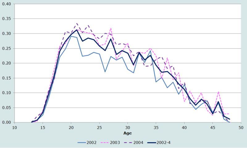
The data vary a lot between calendar years, with estimates of total fertility differing by more than a child per woman between 2002 and 2003. The estimate of total fertility in 2004, despite being derived from only partial exposure in that year for most women is highly consistent with the estimate for 2003. The shape of the distribution (as can be seen in Figure 1) is consistent across the three years, even measured in single years of age. This is true despite a high degree of variability in the estimates by single years of age even if they are aggregated over the three years from 2002 to 2004.
Further aggregating the data into conventional five-year age groups produces the results shown in Table 5.
Table 5 Age-specific fertility rates by grouped year of age and calendar year, Malawi, 2004 DHS
| Age group |
2002 |
2003 |
2004 |
2002-4 |
DHS |
|
15-19 |
0.151 |
0.180 |
0.178 |
0.169 |
0.162 |
|
20-24 |
0.254 |
0.304 |
0.312 |
0.290 |
0.293 |
|
25-29 |
0.210 |
0.261 |
0.283 |
0.252 |
0.254 |
|
30-34 |
0.204 |
0.235 |
0.222 |
0.221 |
0.222 |
|
35-39 |
0.129 |
0.180 |
0.184 |
0.164 |
0.163 |
|
40-44 |
0.075 |
0.078 |
0.086 |
0.080 |
0.080 |
|
45-49 |
0.042 |
0.049 |
0.021 |
0.036 |
0.035 |
|
Total Fertility |
5.32 |
6.44 |
6.43 |
6.05 |
6.05 |
|
Note: 3 year rates as presented in the 2004 DHS report. |
|||||
The differences in the last two columns between the ASFRs derived here and those reported in the DHS survey are very small. However, the much lower fertility rates for 2002 (and 2001, not shown) should give cause for concern about possible reference period errors and shifting of births.
References
Cleland J. 1996. "Demographic data collection in less developed countries", Population Studies 50(3):433-450. doi: https://dx.doi.org/10.1080/0032472031000149556
Rutstein S and G Rojas. 2003. Guide to DHS Statistics. Calverton, MD: ORC Macro.
Schoumaker B. 2010. "Reconstructing fertility trends in sub-Saharan Africa by combining multiple surveys affected by data quality problems " Paper presented at Population Association of America 2010 Annual Meeting. Dallas, TX, April 15-17, 2010.
Schoumaker B. 2011. "Omissions of births in DHS birth histories in sub-Saharan Africa: Measurement and determinants " Paper presented at Population Association of America 2011 Annual Meeting. Washington D.C., March 31 - April 2, 2011.
Schoumaker B. 2013. “A Stata module for computing fertility rates and TFRs from birth histories: tfr2”, Demographic Research 28(Article 38):1093–1144. doi: https://doi.org/10.4054/DemRes.2013.28.38
- Printer-friendly version
- Log in to post comments